Introduction to causal reasoning with graphical models
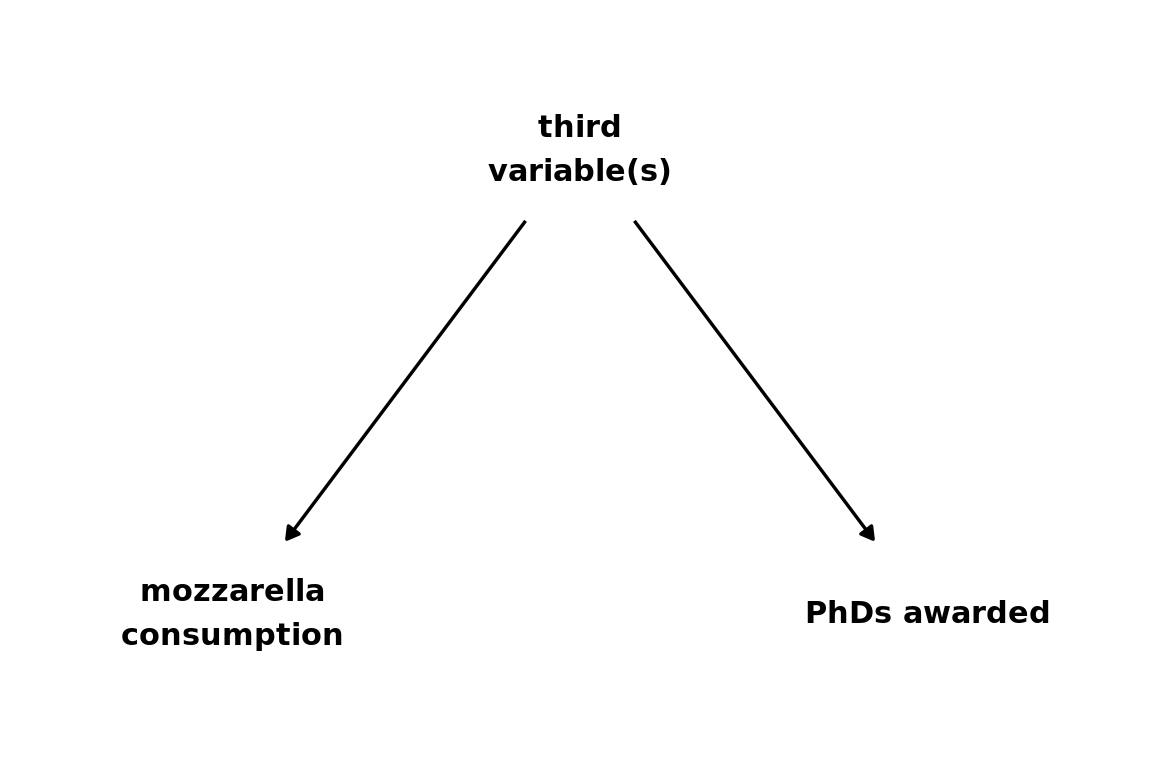
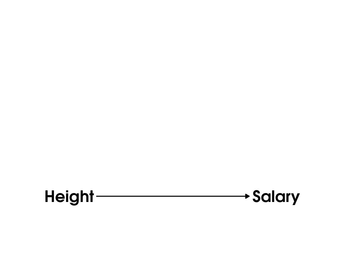
Correlation does not imply causation!
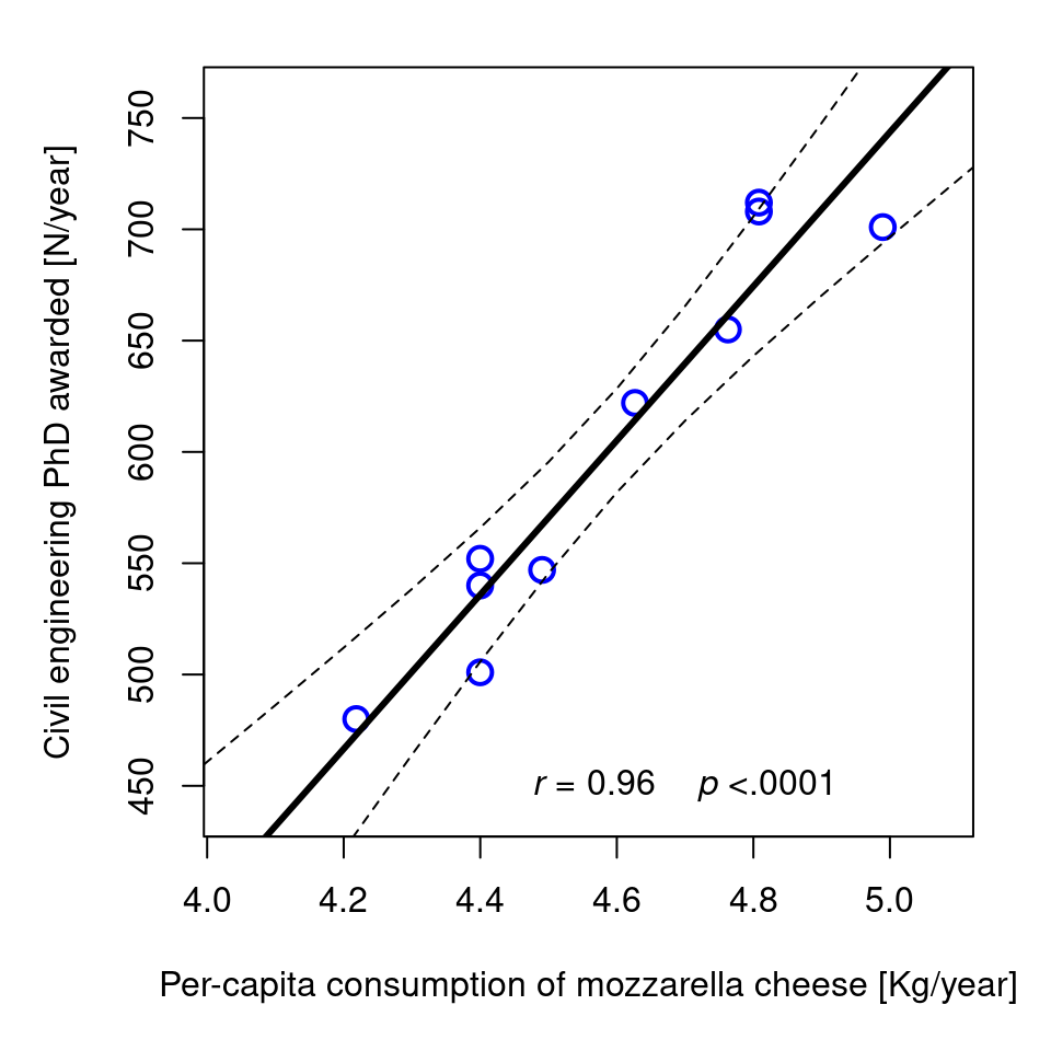
Civil engineering doctorates awarded (in the US; source NSF) as a function of the per capita consumption of mozzarella cheese, measured from 2000 to 2009.
Characterising the role of neurons for behavior is a causal inference question.
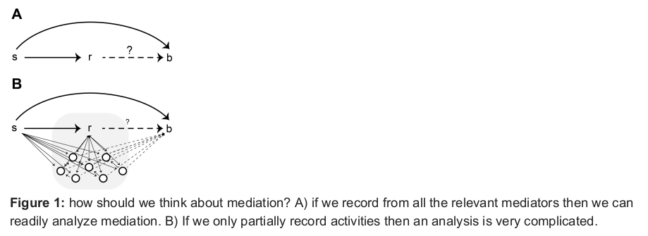
- Neural activity in LIP area was widely believed to causally mediate evidence accumulation in perceptual decision, until it was found it’s pharmacological inactivation had no effect on behavioural performance (Katz et al, Nature 2016)
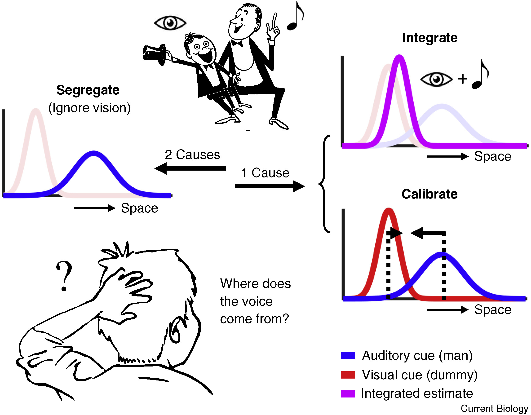
Our sensory system routinely make inferences about causes of the sensory signals it receives.
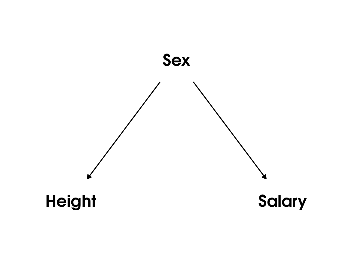
Common cause principle
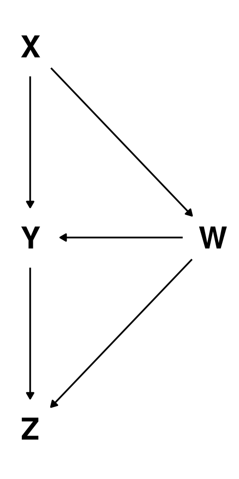
Graphical definitions of causality
A parent variable is a direct cause of it’s child variables
(\(X\) is a direct cause of \(Y\)).An ancestor variable is an indirect or potential cause of its descendants
(\(X\) is a potential cause of \(Z\)).

Acyclicity in DAGs
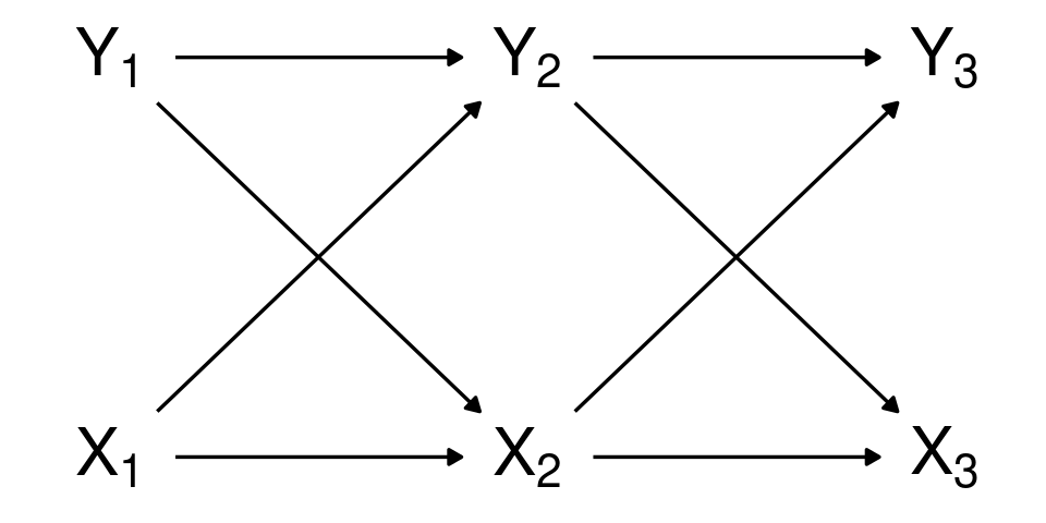
Acyclicity may seem problematic in presence of feedback loops.
One way to deal with these is by adding nodes for repeated measures (e.g. crossed-lagged panel models)
“Structural” errors
Each variable in a DAG is usually assumed to be observed with some error (\(\epsilon_W, \epsilon_X, \ldots\)).
These errors are assumed to be independent from each other, and are usually not shown for simplicity
“The disturbance terms represent independent background factors that the investigator chooses not to include in the analysis” (Pearl, 2009)
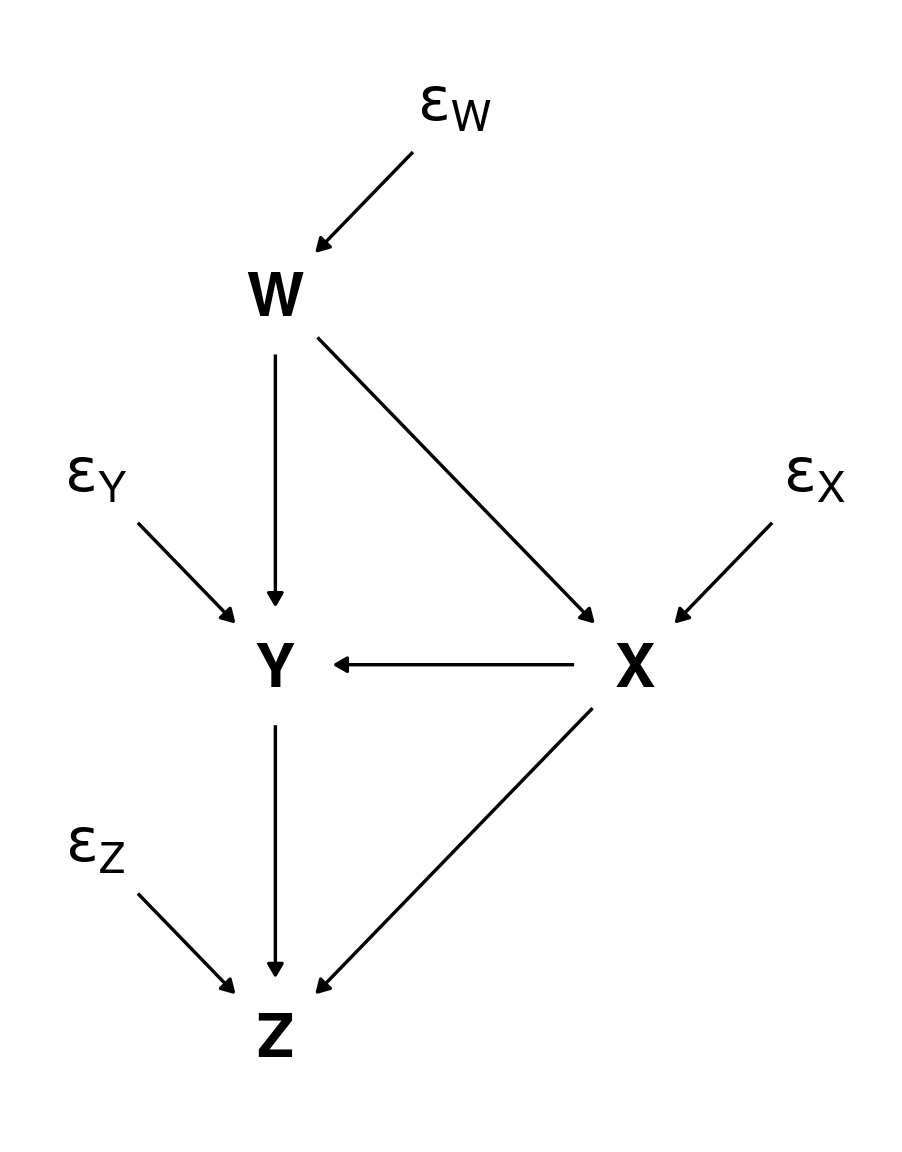
Product decomposition in DAGs
We can write the joint distribution of all variables in a DAG as the product of the conditional distributions \(p(\text{child} \mid \text{parents})\)
\[\begin{align*}p & (X, Y,W,Z) =\\ & p(Z∣W,Y) \, p(Y∣X,W) \, p(W∣X) \, p(X) \end{align*}\]
This holds regardless of the precise functional form of each “arrows”.
A DAG provides a blueprint defining a family of joint probability distributions over a set of variables.

What does “conditioning on a variable” means?
Conditioning on a variable here can be understood as controlling for it.
Conditioning on \(Z\) when studying the link between \(X\) and \(Y\) means we introduce information about \(Z\) in our analysis and ask if \(X\) provide any additional information (above and beyond what we already have knowing \(Z\)).
\[Y \perp\!\!\!\perp X \mid Z\]
How to condition on / control for a variable in practice?
Stratified analysis
Inclusion as covariate in regression models
Matching
All methods of statistical control are affected by measurement errors in confounding variables.
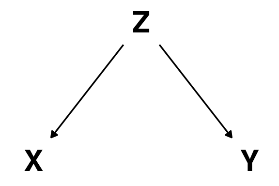
Confounding
Confounding
Colliders
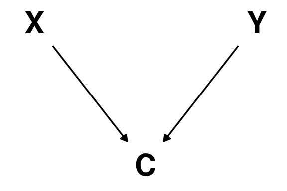
\(X\) and \(Y\) are independent of each other \(X \perp\!\!\!\perp Y\)
\(C\) is caused by both \(X\) and \(Y\)
They become dependent after we condition on the collider node \(C\);
(\(A \not\!\perp\!\!\!\perp B \mid C\))
Cake competition example
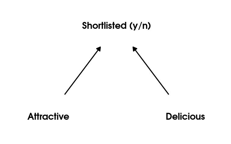
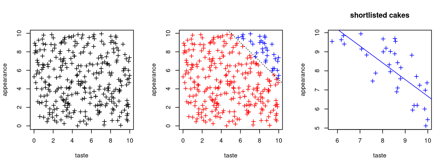
No association between
appearanceandtastein the ‘population’ of cakesappearanceandtastebecomes negatively correlated once we condition our analysis on whether a cake was shortlisted or not.
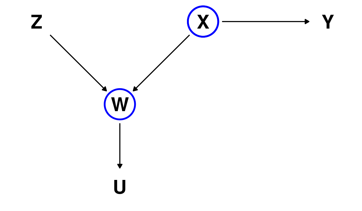
D-separation: example
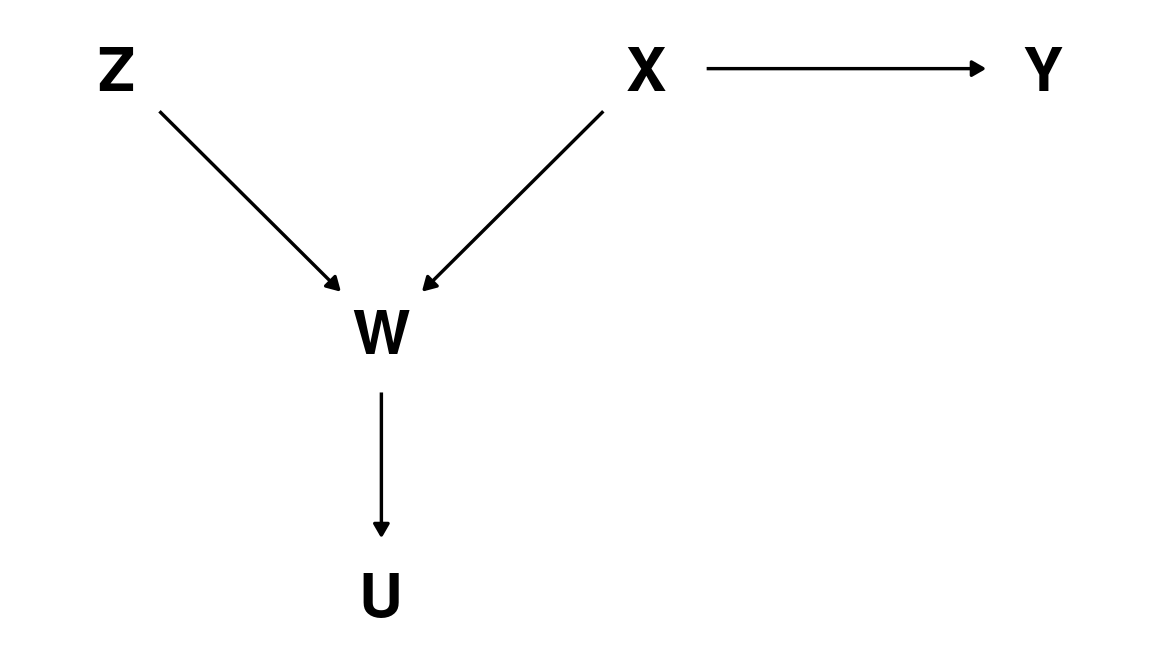
\(Z\) and \(Y\) are D-separated (unconditionally independent, \(Z \perp\!\!\!\perp Y\))
D-separation: example
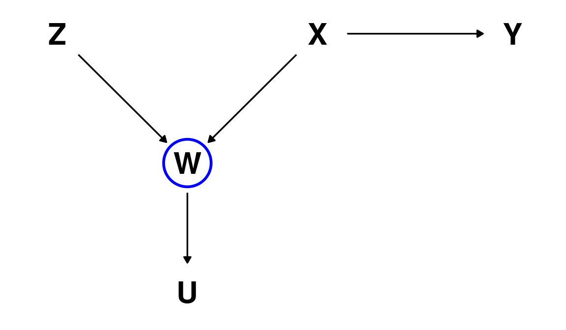
However, \(W\) is a collider node, so if we condition our analysis on \(W\) we would find a ‘spurious’ association between \(Z\) and \(Y\)
This association is ‘spurious’ because \(Y\) is not a descendant of \(Z\).
If we were to make an intervention on \(Z\) this would have no effect on \(Y\).
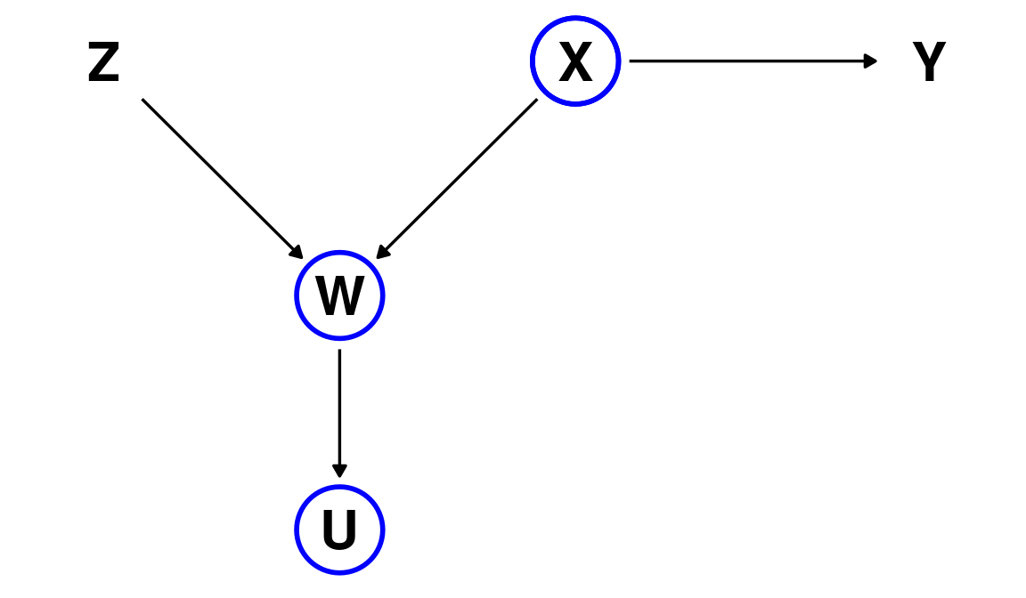
D-separation: example
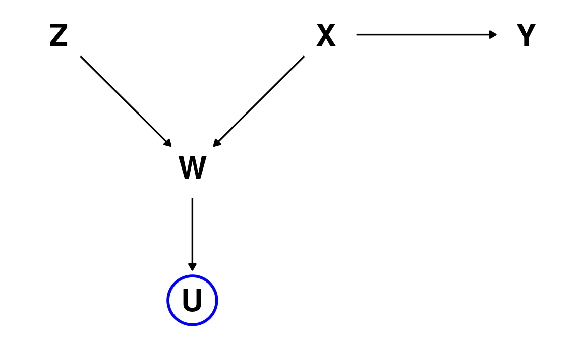
Conditioning on \(U\), the child of the collider node produces the same effect!
(formally \(Z \not\!\perp\!\!\!\perp Y \mid U\))
D-separation: example 2
Which variables that are D-separated (unconditionally independent) in this DAG?
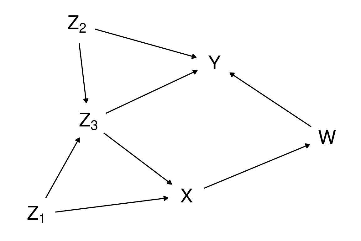
Only \(Z_1\) and \(Z_2\) are unconditionally independent ( \(Z_1 \perp\!\!\!\perp Z_2\)).
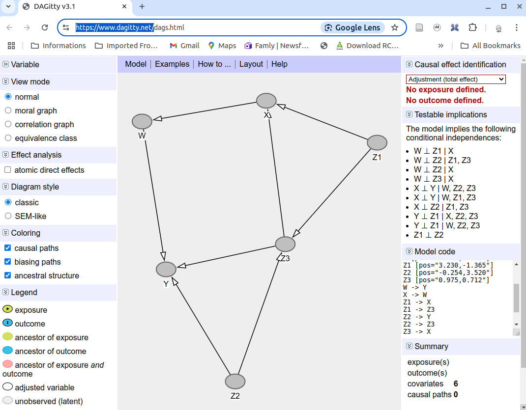
D-separation: example 2
Conditional on which variables are \(Z_1\) and \(W\) independent one another?

Conditioning on \(X\) makes \(Z_1\) and \(W\) independent one another (\(W \perp\!\!\!\perp Z_1 \mid X\)); all other paths are “blocked” by a collider.
Automatic analysis of DAGs with dagitty
D-separation: example 1 again
What happens if we condition on both \(W\) and \(X\)?
Conditioning on \(\{ W,X \}\) makes \(Z\) and \(Y\) conditionally independent.
\(Z \perp\!\!\!\perp Y \mid \{ W,X \}\)
D-separation: example 1 again
As complexity increases the answer is less and less intuitive.
Luckily these questions can be addressed by mechanically applying logical rules, which have been automated in software like dagitty
Blocking confounding paths
To estimate the causal effect of some variable \(X\) to some outcome \(Y\), we need to block all “spurious” paths transmitting non-causal associations
Non-causal paths are essentially paths that connect \(X\) to \(Y\) but have an arrow that enters \(X\). These are non-causal because changing \(X\) will not cause a change in \(Y\) (at least not through this path).
Example:
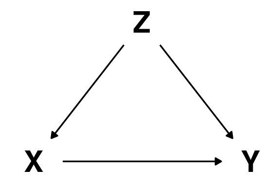
- \(X \in \{0,1\}\) is a binary treatment (e.g., an intervention to improve well-being).
- \(Y \in \{0, 1\}\) is a binary outcome (e.g., whether well-being improves).
- \(Z\) is a confounder that causally influences both the likelihood of receiving the treatment and the chance of well-being improving.
Interventions as ‘surgery’ on graphical models
To estimate the causal effect \(X \rightarrow Y\) we can do a randomized control trial (RCT) in which we allocate people to treatment (\(X = 1\)) and control groups (\(X = 0\)) randomly.
The random allocation can be represented as the deletion of an arrow in the DAG.

If we don’t intervene, the confounder \(Z\) influence the likelihood of taking part in the intervention (\(X\))
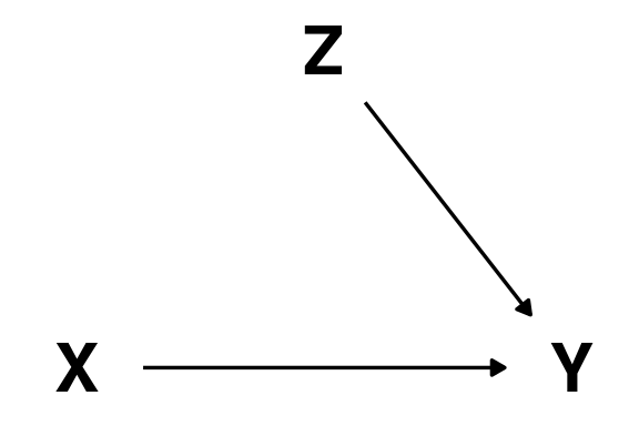
If we intervene on \(X\) by allocating participants randomly we effectively erase the arrow from \(Z\) to \(X\).
In an RCT we can estimate the causal effect simply by measuring the association between \(X\) and \(Y\).
Alternatively (if we can’t intervene) we need block the non-causal path \(X \leftarrow Z \rightarrow Y\) by “controlling” for \(Z\).
To estimate a variable’s causal effect we adjust for its parents in the DAG.
The ‘backdoor’ criterion: example
Here \(X\) is the exposure of interest, \(Y\) the outcome, and \(U\) an unobserved (latent) variable.

There are two ‘indirect’ paths between \(X\) and \(Y\)
- \(X \leftarrow U \leftarrow A \rightarrow C \rightarrow Y\)
- \(X \leftarrow U \rightarrow B \leftarrow C \rightarrow Y\)
Path (2) is already blocked by a collider in \(B\). Path (1) needs to be blocked; we can’t condition on \(U\) since is not observed, so this leaves us either \(A\) or \(C\) (either will suffice).
The ‘backdoor’ criterion: example
The solution can also be found automatically using dagitty:
