Mathematics of 3D eye movements

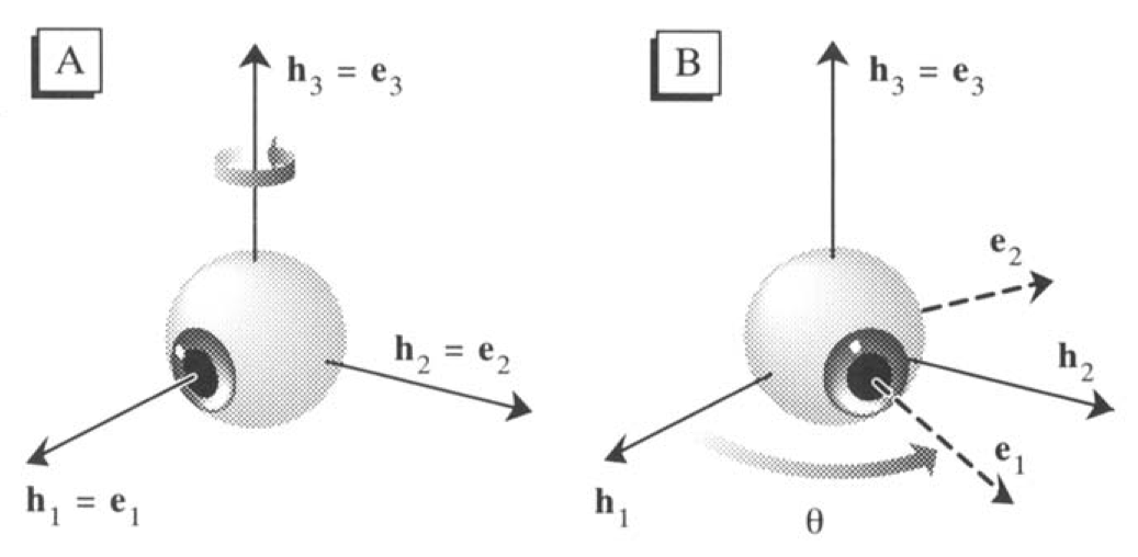
3D eye position can be specified by characterising the 3D rotation that brings the eye to the current eye position from an arbitrary reference or primary position¹, which typically is defined as the position that the eye assumes when looking straight ahead with the head in normal, upright position. This rotation can be described by the 3-by-3 rotation matrix \(\bf{R}\). More specifically the matrix can be used to describe the rotation of three-dimensional coordinates by a certain angle about a certain axis. To formally define this matrix, consider the coordinate system \(\{ \vec{h}_1,\vec{h}_2,\vec{h}_3 \}\) (a coordinate system is defined by a set of linearly independent vectors; e.g. here \(\vec{h}_1 = (1,0,0)\), corresponding to the \(x\) axis) as the head-centered coordinate system where the axis \(\vec{h}_1\) correspond to the visual axis when the eye is in the reference position, and \(\{\vec{e}_1,\vec{e}_2,\vec{e}_3\}\) is an eye-centered coordinate system where \(\vec{e}_1\) always correspond to the visual axis, regardless of the orientation of the eye (see the figure on top of this page). Any orientation of the eye can be described by a matrix \(\bf{R}\) such that \[ {{\vec{e}}_i} = {\bf{R}} {{\vec{h}}_i} \] where \(i=1,2,3\). This rotation matrix is straightforward for 1D rotations. For example, a purely horizontal rotation of an angle \(\theta\) around the axis \(\vec{h}_3\) is formulated as \[ \bf{R}_3 \left( \theta \right) = \left( {\begin{array}{*{20}{c}} {\cos \theta }&{ - \sin \theta }&0\\ {\sin \theta }&{\cos \theta }&0\\ 0&0&1 \end{array}} \right) \] The first two columns of the matrix indicates the new coordinates of the first (i.e., \(\vec{h}_1\)) and of the second basis (\(\vec{h}_2\)) of the new eye-centerd coordinate system after the rotation, expressed according to the initial head-centered coordinate system. The third basis, \(\vec{h}_3\) is the axis of rotation, and does not change. It becomes more complicated for 3D rotations, i.e. rotations of the fixed eye-centered coordinate system to any new orientation. They can be obtained by calculating a sequence of 3 different rotations about the three fixed axis, and multiplying the corresponding matrices: \(\bf{R} = \bf{R}_3 \left( \theta \right) \bf{R}_2 \left( \phi \right) \bf{R}_1 \left( \psi \right)\). Although the first two rotations are sufficient to specity the orientation of the visual axis, the third is necessary to specify the torsion component and fully specify the 3D orientation of the eye. Importantly, the order of the three rotations is relevant - rotations are not commutative, so if you put them in different order you end up with a different result - and needs to be arbitrarily specified (when it is specified in this order is referred to as Flick sequence). This representation of 3D orientations is not very efficient (9 values, while only 3 are necessary), or practical for computations; additionally one needs to define arbitrarily the order of the rotations of the sequence.

Quaternions and rotation vectors

An alternative way to describe rotations is with quaternions. Quaternions can be looked upon as four-dimensional vectors, although they are more commonly split in a real scalar part and an imaginary vector part; they are in fact an extension of the complex numbers. They have the form \[ q_0 + q_1i + q_2j + q_3k = \left( q_0,\vec{q} \cdot \vec{I} \right) = \left( r,\vec{v} \right) \] where \[ \vec{q} = \left( \begin{array}{*{20}{c}} {q_1}\\ {q_2}\\ {q_3} \end{array} \right) \] and \[ \vec{I} = \left( \begin{array}{*{20}{c}} {i}\\ {j}\\ {k} \end{array} \right) \] \(i,j,k\) are the quaternion units. These can be multiplied according to the following formula, discovered by Hamilton in 1843 \[ i^2 = j^2 = k^2 = ijk = - 1 \] This formula may seems strange but it determines all the possible products of \(i,j,k\), such as \(ij=k\) and \(ji=-k\). Note that the product of the basis are not commutative. There is a visual trick to remember the multiplication rules, based on the following diagram:

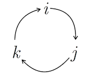
Multiplying quaternions. Multiplying two elements in the clockwise direction gives the next element along the same direction (e.g. \(jk=i\)). The same is for counter-clockwise directions, except that the result is negative (e.g. \(kj=-i\)).

Quaternions can be used to represent rotations. For example, a rotation of an angle \(\theta\) around the axis define by the unit vector \(\vec{u} = (u_1, u_2,u_3) = u_1i + u_2j + u_3k\)² can be described by the following quaternion \[ \cos \frac{\theta}{2} + \sin \frac{\theta}{2}\left( u_1i + u_2j + u_3k \right) \] The direction of the rotation is given by the right-hand rule. Successive rotations can combined using the formula for quaternion multiplication. The multiplication of quaternions can be computed by the products of their elements element as if they were two polynomials, but keeping track of the ordering of the basis, as their multiplication is not commutative. This is a desired property if we want to specify rotations, which as seen earlier are also not commutative. Quaternion multiplication can be also expressed in the modern language of vector and cross product \[ \left( r_1,\vec{v_1} \right) \left( r_2,\vec{v_2} \right) = \left( r_1 r_2 - \vec{v_1} \cdot \vec{v_2},\;\; r_1\vec{v_2} + r_2\vec{v_1} +\vec{v_1} \times \vec{v_2} \right) \] where “\(\cdot\)” is the dot product and “\(\times\)” is the cross product.

In sum, quaternions are pretty useful to compute transformations in 3D. One can use quaternions to combine 3D any sequence of rotations about arbitrary axis (using quaternion multiplications), as well as to rotate any 3D Euclidean vector about any arbitrary axis. A quaternion can also be transformed into a 3D rotation matrix (formula here), which then may be used in 3D graphics.

Rotation vectors are an even more succint representation of rotations. Indeed, the scalar component of the quaterion (\(q_0\)) does not add any information that is not alredy in the vector part, so a rotation could be effectively described by just 3 numbers. The rotation vector \(\vec{r}\), which correspond to a rotation of an angle \(\theta\) about an axis \(\vec{n}\) is defined as \[ \vec{r} = \tan \left( \frac{\theta}{2} \right) \vec{n} \] which can be defined also with respect to the equivalent quaternion \(\textbf{q}\) \[ \textbf{q}=\left( q_0, \vec{q} \right) = \left( \cos \left(\frac{\theta}{2}\right), \sin \left(\frac{\theta}{2}\right)\vec{n} \right) \] as \[ \vec{r} = \frac{\vec{q}}{q_0} \].

Donder’s law and Listing’s law

Donder’s law (1848) states that the eye use only two degrees of freedom while fixating, although mechanically it has three. In othere words this means that the torsion component of the eye movement is not arbitrary but it is uniquely determined by the direction of the visual axis and is independent of the previous eye movements. From the material review above it should be clear how any 3D eye orientation can be fully described as a rotation abour a given axis from a primary reference position. This allows also to formulate Donder’s law more specifically,according to what is known as Listing’s law (Helmholtz et al. 1910,@Haustein1989) “There exists a certain eye position from which the eye may reach any other position of fixation by a rotation around an axis perpendicular to the visual axis. This particular position is called primary position”. This means that all possible eye positions can be reached from the primary position by a single rotation about an axis perpendicular to the visual axis. Since they are all perpendicular to the visual axis, all rotation axis that satisfy Listing’s law are on the same plane (Listing’s plane). The law can be tested with eyetracking equipments that allows measuring also the torsional components (such as scleral coils): results have shown that the standard deviation from Listing’s plane of empirically measured rotation vectors is only about 0.5-1 deg (Haslwanter 1995). Formally it can be written that for any orientation of the visual axis, defined by the rotation vector \(\vec{a}\) and measured from the primary position \(\vec{h_1}=(1,0,0)\), \[ \vec{h_1} \cdot \vec{a} = 0 \] This indicates simply that the rotation about the visual axis is 0, and that as a consequence all the rotation axes lies in a frontal plane.

Going back to the beginning, knowing the coordinates os Listing’s plane one can compute the rotation vector that correspond to the current eye position from the recording of the 2D gaze location on a screen. In the simplest case, we assume that the primary position corresponds to when the observer fixates the center of the screen, \((0,0)\). What is the rotation vector that describes the 3D eye orientation when the observer fixates the location \((s_x, s_y)\) ? Let’s say the position on screen is defined in cm, and we know that the distance of the eye from the screen is \(L\) cm. The rotation angle can be computed as \(\theta = \rm{atan} \frac{\sqrt{s_x^2+s_y^2}}{L}\), while the angle that defines the orientation of the rotation axis within Listing’s plane is \(\alpha = \rm{atan2}(s_y,s_x)\). The complete rotation vector is then \[ \vec{r} = \tan \left( \frac{\theta}{2}\right) \cdot \left( {\begin{array}{*{20}{c}} 0\\ {\cos \alpha }\\ { - \sin \alpha } \end{array}} \right) \] This vector describe aparticular eye position as a rotation from the reference position, and does not have a torsional component (that is a component along \(\vec{h_1}\)). Indeed, Listing’s law implies that all possible eye positions can be reached from the primary reference position without a torsional component. However, vectors describing rotations from and to positions different than the primary one do not, in general, lie in Listing’s plane. For Listing law to hold such vectors must lie in a plane whose orientation depends on the current eye position, and more specifically is such that the vector perpendicular to the plane is exactly halfway between the current and the primary eye position (Tweed and Vilis 1990).

References

Haslwanter, Thomas. 1995. “Mathematics of three-dimensional eye rotations.” Vision Research 35 (12): 1727–39. https://doi.org/10.1016/0042-6989(94)00257-M.
Haustein, Werner. 1989. “Considerations on Listing’s Law and the primary position by means of a matrix description of eye position control.” Biological Cybernetics 60 (6): 411–20. https://doi.org/10.1007/BF00204696.
Helmholtz, Hermann von, Hermann von Helmholtz, Hermann von Helmholtz, and Hermann von Helmholtz. 1910. Handbuch der Physiologischen Optik. Hamburg: Voss.
Tweed, Douglas, and Tutis Vilis. 1990. “Geometric relations of eye position and velocity vectors during saccades.” Vision Research 30 (1): 111–27. https://doi.org/10.1016/0042-6989(90)90131-4.
Euler’s theorem guarantee that a rigid body can always move from one orientation to any different one through a single rotation about a fixed axis.↩
Saying that \(\vec(u)\) is a unit vector indicates that it has length 1, i.e. \(\left| \vec{u} \right| = \sqrt{u_1^2 + u_2^2 + u_3^2} = 1\)↩