
Photo ©Roxie and Lee Carroll, www.akidsphoto.com.
In my previous lab I was known for promoting the use of multilevel, or mixed-effects model among my colleagues. (The slides on the /misc section of this website are part of this effort.) Multilevel models should be the standard approach in fields like experimental psychology and neuroscience, where the data is naturally grouped according to “observational units”, i.e. individual participants. I agree with Richard McElreath when he writes that “multilevel regression deserves to be the default form of regression” (see here, section 1.3.2) and that, at least in our fields, studies not using a multilevel approach should justify the choice of not using it.
In \(\textsf{R}\), the easiest way to fit multilevel linear and generalized-linear models is provided by the lme4 library (Bates et al. 2014). lme4 is a great package, which allows users to test different models very easily and painlessly. However it has also some limitations: it can be used to fit only classical forms of linear and generalized linear models, and can’t, for example, use to fit psychometric functions that take attention lapses into account (see here). Also, lme4 allows to fit multilevel models from a frequentist approach, and thus do not allow to incorporate prior knowledge into the model, or to use regularizing priors to reduce the risk of overfitting. For this reason, I have recently started using Stan, through its \(\textsf{R}\)Stan interface, to fit multilevel models in a Bayesian settings, and I find it great! It certainly requires more effort to define the models, however I think that the flexibility offered by a software like Stan is well worth the time spent to learning how to use it.
For people like me, used to work with lme4, Stan can be a bit discouraing at first. The approach to write the model is quite different, and it requires specifying explicitly all the distributional assumptions. Also, implementing models with correlated random effects requires some specific notions of algebra. So I prepared a first tutorial showing how to analyse in Stan one of the most common introductory examples to mixed-effects models, the sleepstudy dataset (contained in the lme4 package). This will be followed by another tutorial showing how to use this approach to fit dataset where the dependent variable is a binary outcome, as it is the case for most psychophysical data.
The sleepstudy example
This dataset contains part of the data from a published study (Belenky et al. 2003) that examined the effect of sleep deprivation on reaction times. (This is a sensible topic: think for example to long-distance truck drivers.) The dataset contains the average reaction times for the 18 subjects of the sleep-deprived group, for the first 10 days of the study, up to the recovery period.
library(lme4)
Loading required package: Matrix
str(sleepstudy)
'data.frame':   180 obs. of  3 variables:
 $ Reaction: num  250 259 251 321 357 ...
 $ Days    : num  0 1 2 3 4 5 6 7 8 9 ...
 $ Subject : Factor w/ 18 levels "308","309","310",..: 1 1 1 1 1 1 1 1 1 1 ...
The model I want to fit to the data will contain both random intercepts and slopes; in addition the correlation between the random effects should also be estimated. Using lme4, this model could be estimated by using
lmer(Reaction ~ Days + (Days | Subject), sleepstudy)The model could be formally notated as \[ y_{ij} = \beta_0 + u_{0j} + \left( \beta_1 + u_{1j} \right) \cdot {\rm{Days}} + e_i \] where \(\beta_0\) and \(\beta_1\) are the fixed effects parameters (intercept and slope), \(u_{0j}\) and \(u_{1j}\) are the subject specific random intercept and slope (the index \(j\) denotes the subject), and \(e \sim\cal N \left( 0,\sigma_e^2 \right)\) is the (normally distributed) residual error. The random effects \(u_0\) and \(u_1\) have a multivariate normal distribution, with mean 0 and covariance matrix \(\Omega\) \[ \left[ {\begin{array}{*{20}{c}} {{u_0}}\\ {{u_1}} \end{array}} \right] \sim\cal N \left( {\left[ {\begin{array}{*{20}{c}} 0\\ 0 \end{array}} \right],\Omega = \left[ {\begin{array}{*{20}{c}} {\sigma _0^2}&{{\mathop{\rm cov}} \left( {{u_0},{u_1}} \right)}\\ {{\mathop{\rm cov}} \left( {{u_0},{u_1}} \right)}&{\sigma _1^2} \end{array}} \right]} \right) \]
In Stan, fitting this model requires preparing a separate text file (usually saved with the ‘.stan’ extension), containing several “blocks”. The 3 main types of blocks in Stan are:
dataall the dependent and independent variables needs to be declared in this blocksparametershere one should declare the free parameters of the model; what Stan do is essentially use a MCMC algorithm to draw samples from the posterior distribution of the parameters given the datasetmodelhere one should define the likelihood function and, if used, the priors
Additionally, we will use two other types of blocks, transformed parameters and generated quantities. The first is necessary because we are estimating also the full correlation matrix of the random effects. We will parametrize the covariance matrix as the Cholesky factor of the correlation matrix (see my post on the Cholesky factorization), and in the transformed parameters block we will multiply the random effects with the Choleki factor, to transform them so that they have the intended correlation matrix. The generated quantities block can be used to compute any additional quantities we may want to compute once for each sample; I will use it to transform the Cholesky factor into the correlation matrix (this step is not essential but makes the examination of the model easier).
Data
RStan requires the data to be organized in a list object. It can be done with the following command
d_stan <- list(Subject = as.numeric(factor(sleepstudy$Subject,
    labels = 1:length(unique(sleepstudy$Subject)))), Days = sleepstudy$Days,
    RT = sleepstudy$Reaction/1000, N = nrow(sleepstudy), J = length(unique(sleepstudy$Subject)))
Note that I also included two scalar variables, N and J, indicating respectively the number of observation and the number of subjects. Subject was a categorical factor, but to input it in Stan I transformed it into an integer index. I also rescaled the reaction times, so that they are in seconds instead of milliseconds.
These variables can be declared in Stan with the following block. We need to declare the variable type (e.g. real or integer, similarly to programming languages as C++) and for vectors we need to declare the length of the vectors (hence the need of the two scalar variables N and J). Note that variables can be given lower and upper bounds. See the Stan reference manual for more information of the variable types.
data {
  int<lower=1> N;            //number of observations
  real RT[N];                //reaction times

  int<lower=0,upper=9> Days[N];   //predictor (days of sleep deprivation)

  // grouping factor
  int<lower=1> J;                   //number of subjects
  int<lower=1,upper=J> Subject[N];  //subject id
}
Parameters
Here is the parameter block. Stan will draw samples from the posterior distribution of all the parameters listed here. Note that for parameters representing standard deviations is necessary to set the lower bound to 0 (variances and standard deviations cannot be negative). This is equivalent to estimating the logarithm of the standard deviation (which can be both positive or negative) and exponentiating before computing the likelihood (because \(e^x>0\) for any \(x\)). Note that we have also one parameter for the standard deviation of the residual errors (which was implicit in lme4).
The random effects are parametrixed by a 2 x J random effect matrix z_u, and by the Cholesky factor of the correlation matrix L_u. I have added also the transformed parameters block, where the Cholesky factor is first multipled by the diagonal matrix formed by the vector of the random effect variances sigma_u, and then is multiplied with the random effect matrix, to obtain a random effects matrix with the intended correlations, which will be used in the model block below to compute the likelihood of the data.
parameters {
  vector[2] beta;                   // fixed-effects parameters
  real<lower=0> sigma_e;            // residual std
  vector<lower=0>[2] sigma_u;       // random effects standard deviations

  // declare L_u to be the Choleski factor of a 2x2 correlation matrix
  cholesky_factor_corr[2] L_u;

  matrix[2,J] z_u;                  // random effect matrix
}

transformed parameters {
  // this transform random effects so that they have the correlation
  // matrix specified by the correlation matrix above
  matrix[2,J] u;
  u = diag_pre_multiply(sigma_u, L_u) * z_u;

}
Model
Finally the model block. Here we can define priors for the parameters, and then write the likelihood of the data given the parameters. The likelihood function corresponds to the model equation we saw before.
model {
  real mu; // conditional mean of the dependent variable

  //priors
  L_u ~ lkj_corr_cholesky(1.5); // LKJ prior for the correlation matrix
  to_vector(z_u) ~ normal(0,2);
  sigma_e ~ normal(0, 5);       // prior for residual standard deviation
  beta[1] ~ normal(0.3, 0.5);   // prior for fixed-effect intercept
  beta[2] ~ normal(0.2, 2);     // prior for fixed-effect slope

  //likelihood
  for (i in 1:N){
    mu = beta[1] + u[1,Subject[i]] + (beta[2] + u[2,Subject[i]])*Days[i];
    RT[i] ~ normal(mu, sigma_e);
  }
}
For the correlation matrix, Stan manual suggest to use a LKJ prior1. This prior has one single shape parameters, \(\eta\): if you set \(\eta=1\) then you have effectively a uniform prior distribution over any (Cholesky factor of) 2x2 correlation matrices. For values \(\eta>1\) instead you get a more conservative prior, with a mode in the identity matrix (where the correlations are 0). For more information about the LKJ prior see page 556 of Stan reference manual, version 2.17.0, and also this page for an intuitive demonstration.
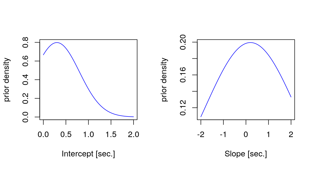
Importantly, I have used (weakly) informative priors for the fixed effect estimates. We know from the literature that simple reaction times are around 300ms, hence the prior for the intercept, which represents the avearage reaction times at Day 0, i.e. before the sleep deprivation. We expect the reaction times to increase with sleep deprivation, so I have used for the slope a Gaussian prior centered at a small positive value (0.2 seconds), which would represents the increase in reaction times with each day of sleep deprivation, however using a very broad standard deviation (2 seconds), which could accomodate also negative or very different slope values if needed. It may be useful to visualize with a plot the priors.
Generated quantities
Finally, we can add one last block to the model file, to store for each sampling iteration the correlation matrix of the random effect, which can be computed multyplying the Cholesky factor with its transpose.
generated quantities {
  matrix[2, 2] Omega;
  Omega = L_u * L_u'; // so that it return the correlation matrix
}
Estimating the model
Having written all the above blocks in a separate text file (I called it “sleep_model.stan”), we can call Stan from R with following commands. I run 4 independent chains (each chain is a stochastic process which sequentially generate random values; they are called chain because each sample depends on the previous one), each for 2000 samples. The first 1000 samples are the warmup (or sometimes called burn-in), which are intended to allow the sampling process to settle into the posterior distribution; these samples will not be used for inference. Each chain is independent from the others, therefore having multiple chains is also useful to check the convergence (i.e. by looking if all chains converged to the same regions of the parameter space). Additionally, having multiple chain allows to compute a statistic which is also used to check convergence: this is called \(\hat R\) and it corresponds to the ratio of the between-chain variance and the within-chain variance. If the sampling has converged then \({\hat R} \approx 1 \pm 0.01\).
When we call function stan, it will compile a C++ program which produces samples from the joint posterior of the parameter using a powerful variant of MCMC sampling, called Hamiltomian Monte Carlo (see here for an intuitive explanation of the sampling algorithm).
library(rstan)
options(mc.cores = parallel::detectCores())  # indicate stan to use multiple cores if available
sleep_model <- stan(file = "sleep_model.stan", data = d_stan,
    iter = 2000, chains = 4)
One way to check the convergence of the model is to plot the chain of samples. They should look like a “fat, hairy caterpillar which does not bend” (Sorensen, Hohenstein, and Vasishth 2016), suggesting that the sampling was stable at the posterior.
traceplot(sleep_model, pars = c("beta"), inc_warmup = FALSE)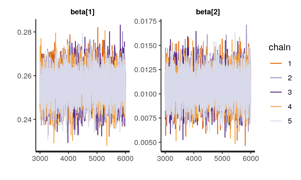 There is a
 print() method for visualising the estimates of the parameters. The values of the \({\hat R}\) (Rhat) statistics also confirm that the chains converged. The method automatically report credible intervals for the parameters (computed with the percentile method from the samples of the posterior distribution).
print(sleep_model, pars = c("beta"), probs = c(0.025, 0.975),
    digits = 3)
Inference for Stan model: sleep_model_v1.
5 chains, each with iter=6000; warmup=3000; thin=1;
post-warmup draws per chain=3000, total post-warmup draws=15000.

         mean se_mean    sd  2.5% 97.5% n_eff Rhat
beta[1] 0.255       0 0.006 0.243 0.268  6826    1
beta[2] 0.011       0 0.001 0.008 0.013  7830    1

Samples were drawn using NUTS(diag_e) at Sat Sep 22 17:15:42 2018.
For each parameter, n_eff is a crude measure of effective sample size,
and Rhat is the potential scale reduction factor on split chains (at
convergence, Rhat=1).
And we can visualze the posterior distribution as histograms (here for the fixed effects parameters and the standard deviations of the corresponding random effects).
plot(sleep_model, plotfun = "hist", pars = c("beta", "sigma_u"))
`stat_bin()` using `bins = 30`. Pick better value with `binwidth`.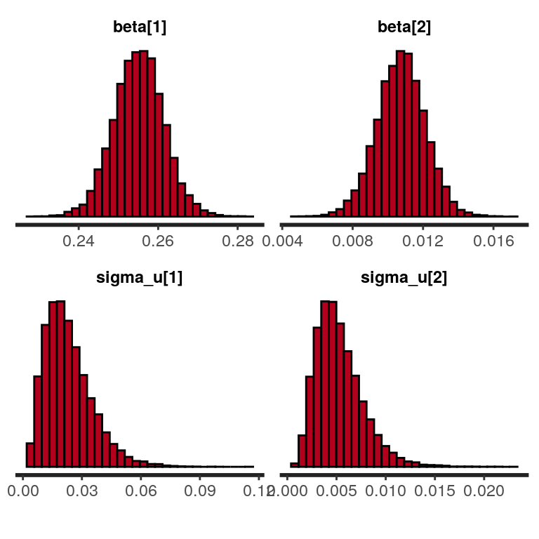 Finally, we can also examine the correlation matrix of random-effects.
print(sleep_model, pars = c("Omega"), digits = 3)
Inference for Stan model: sleep_model_v1.
5 chains, each with iter=6000; warmup=3000; thin=1;
post-warmup draws per chain=3000, total post-warmup draws=15000.

            mean se_mean    sd   2.5%   25%   50%   75% 97.5% n_eff  Rhat
Omega[1,1] 1.000     NaN 0.000  1.000 1.000 1.000 1.000 1.000   NaN   NaN
Omega[1,2] 0.221   0.007 0.344 -0.546 0.011 0.251 0.467 0.807  2228 1.001
Omega[2,1] 0.221   0.007 0.344 -0.546 0.011 0.251 0.467 0.807  2228 1.001
Omega[2,2] 1.000   0.000 0.000  1.000 1.000 1.000 1.000 1.000   160 1.000

Samples were drawn using NUTS(diag_e) at Sat Sep 22 17:15:42 2018.
For each parameter, n_eff is a crude measure of effective sample size,
and Rhat is the potential scale reduction factor on split chains (at
convergence, Rhat=1).
The Rhat values for the first entry of the correlation matrix is NaN. This is expected for variables that remain constant during samples. We can check that this variable resulted in a series of identical values during sampling with the following command
all(unlist(extract(sleep_model, pars = "Omega[1,1]")) == 1)  # all values are =1 ?
[1] TRUE
That’s all! You can check by yourself that the values are the sufficiently similar to what we would obtain using lmer, and eventually experiment by yourself how the estimates changes when more informative priors are used. For more examples on how to fit linear mixed-effects models using Stan I recommend the article by Sorensen (Sorensen, Hohenstein, and Vasishth 2016), which also show how to implement crossed random effects of subjects and item (words), as it is conventional in linguistics.
References
Bates, D, M Maechler, B Bolker, and S Walker. 2014. “lme4: Linear mixed-effects models using Eigen and S4.” R package version 1.1-7. http://cran.r-project.org/package=lme4.
Belenky, Gregory, Nancy J Wesensten, David R Thorne, Maria L Thomas, Helen C Sing, Daniel P Redmond, Michael B Russo, and J Balkin, Thomas. 2003. “Patterns of performance degradation and restoration during sleep restriction and subsequent recovery: a sleep dose-response study.” Journal of Sleep Research 12 (1): 1–12. https://doi.org/10.1046/j.1365-2869.2003.00337.x.
Sorensen, Tanner, Sven Hohenstein, and Shravan Vasishth. 2016. “Bayesian linear mixed models using Stan: A tutorial for psychologists, linguists, and cognitive scientists.” The Quantitative Methods for Psychology 12 (3): 175–200. https://doi.org/10.20982/tqmp.12.3.p175.
The LKJ prior is named after the authors, see: Lewandowski, D., Kurowicka, D., and Joe, H. (2009). Generating random correlation matrices based on vines and extended onion method. Journal of Multivariate Analysis, 100:1989–2001↩