In experimental psychology and neuroscience the classical approach when comparing different models that make quantitative predictions about the behavior of participants is to aggregate the predictive ability of the model (e.g. as quantified by Akaike Information criterion) across participants, and then see which one provide on average the best performance. Although correct, this approach neglect the possibility that different participants might use different strategies that are best described by alternative, competing models. To account for this, Stephan et al. (Stephan et al. 2009) proposed a more conservative approach where models are treated as random effects that could differ between subjects and have a fixed (unknown) distribution in the population. The relevant statistical quantity is the frequency with which any model prevails in the population. Note that this is different from the definition of random-effects in classical statistic where random effects models have multiple sources of variation, e.g. within- and between- subject variance. An useful and popular way to summarize the results of this analysis is by reporting the model’s exceedance probabilities, which measures how likely it is that any given model is more frequent than all other models in the set. The following exposition is largerly based on Stephan et al’s paper (Stephan et al. 2009).
Model evidence
Let’s say we have an experiment with \(\left(1,\dots,N\right)\) participants. Their performance is quantitatively predicted by a set \(\left(1,\dots,K\right)\) competing models. The behaviour of any subject \(n\) can be fit by the model \(k\) by finding the value(s) of the parameter(s) \(\theta_k\) that maximize the likelihood of the data \(y_n\) under the model. In a fully Bayesian setting each unknown parameter would have a prior probability distribution, and the quantity of choice ofr comparing the goodness of fit of the model is the marginal likelihood, that is \[ p \left(y_n \mid k \right) = \int p\left(y_n \mid k, \theta_k \right) \, p\left(\theta_k \right) d\theta. \] By integrating over the prior probability of parameters the marginal likelihood provide a measure of the evidence in favour of a specific model while taking into account the complexity of the model. We might also do something simpler and approximate the model evidence using e.g. the Akaike information criterion.
Models as random effects
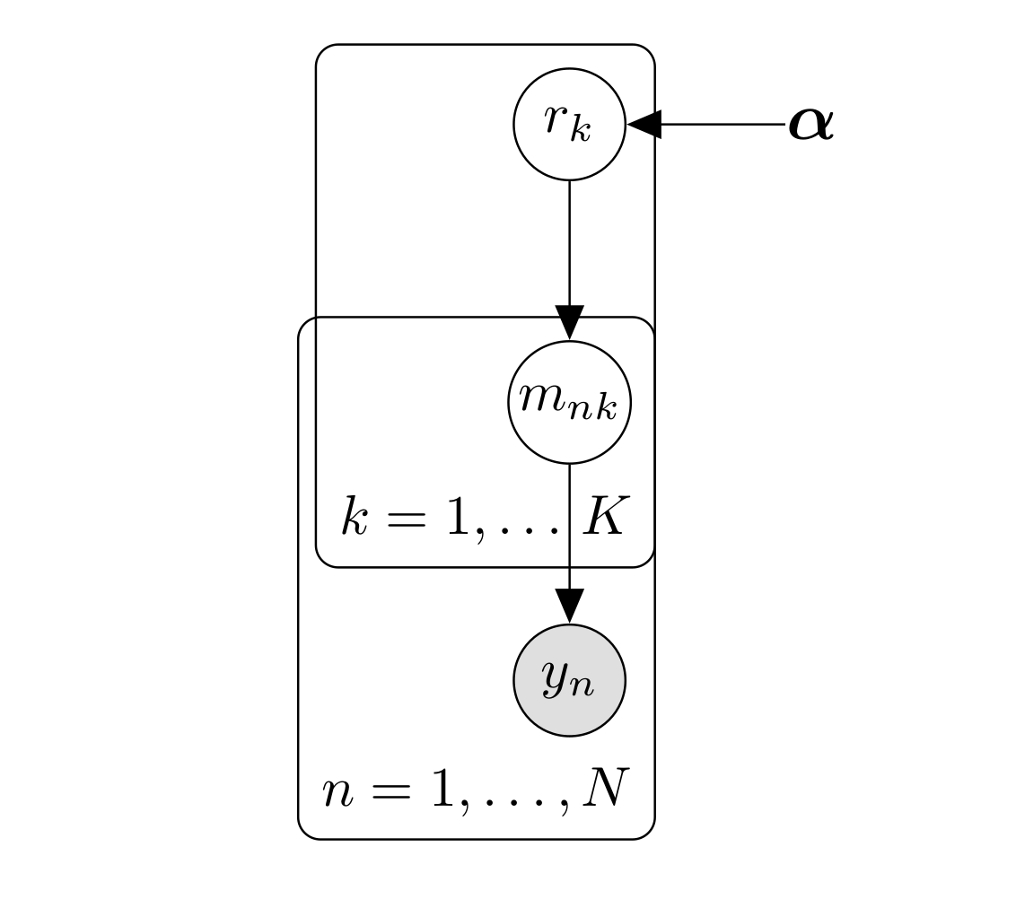
We are interested in finding which model does better at predicting behavior, however we allow for different participants to use different strategies which can be represented by different models. To achieve that we treat the model as random effects and we assume that the frequency or probability of models in the population, \((r_1, \dots, r_K)\), is described by a Dirichlet distribution with parameters \(\boldsymbol{\alpha } = \alpha_1, \dots, \alpha_k\), \[ \begin{align} p\left(r \mid \boldsymbol{\alpha } \right) & = \text{Dir} \left(r, \boldsymbol{ \alpha } \right) \\ & = \frac{1}{\mathbf{B} \left(\boldsymbol{ \alpha } \right)} \prod_{i=1}^K r_i^{\alpha_i -1} \nonumber \end{align}. \] Where the normalizing constant \(\mathbf{B} \left(\boldsymbol{ \alpha } \right)\) is the multivariate Beta function. The probabilities \(r\) generates ‘switches’ or indicator variables \(m_n = m_1, \dots, m_N\) where \(m \in \left \{ 0, 1\right \}\) and \(\sum_1^K m_{nk}=1\). These indicator variables prescribe the model for the subjects \(n\), $ p(m_{nk}=1)=r_k$. Given the probabilities \(r\), the indicator variables have thus a multinomial distribution, that is \[ p\left(m_n \mid \mathbf{r} \right) = \prod_{k=1}^K r_k^{m_{nk}}. \] The graphical model that summarizes these dependencies is shown the following graph:
Variational Bayesian approach
The goal is to estimate the parameters \(\boldsymbol{\alpha}\) that define the posterior distribution of model frequencies given the data, $ p ( r | y)$. To do so we need an estimate of the model evidence \(p \left(m_{nk}=1 \mid y_n \right)\), that is the belief that the model \(k\) generated data from subject \(m\). There are many possible approach that can be used to estimate the model evidence, either exactly or approximately. Importantly, these would need to be normalized so that they sum to one across models, so that is one were using the Akaike Information criterion, this should be transformed into Akaike weights (Burnham and Anderson 2002).
Generative model
Given the graphical model illustrated above, the joint probability of parameters and data can be expressed as \[ \begin{align} p \left( y, r, m \right) & = p \left( y \mid m \right) \, p \left( m \mid r \right) \, p \left( r \mid \boldsymbol{\alpha} \right) \\ & = p \left( r \mid \boldsymbol{\alpha} \right) \left[ \prod_{n=1}^N p \left( y_n \mid m_n \right) \, p\left(m_n \mid r \right) \right] \nonumber \\ & = \frac{1}{\mathbf{B} \left(\boldsymbol{ \alpha } \right)} \left[ \prod_{k=1}^K r_k^{\alpha_k -1} \right] \left[ \prod_{n=1}^N p \left( y_n \mid m_n\right) \, \prod_{k=1}^K r_k^{m_{nk}} \right] \nonumber \\ & = \frac{1}{\mathbf{B} \left(\boldsymbol{ \alpha } \right)} \prod_{n=1}^N \left[ \prod_{k=1}^K \left[ p \left( y_n \mid m_{nk} \right) \, r_k \right]^{m_{nk}} \, r_k^{\alpha_k -1} \right]. \nonumber \end{align} \] And the log probability is \[ \log p \left( y, r, m \right) = - \log \mathbf{B} \left(\boldsymbol{ \alpha } \right) + \sum_{n=1}^N \sum_{k=1}^K \left[ \left(\alpha_k -1 \right) \log r_k + m_{nk} \left( p \left( \log y_n \mid m_{nk} \right) + \log r_k\right)\right]. \]
Variational approximation
In order to fit this hierarchical model following the variational approach one needs to define an approximate posterior distribution over model frequencies and assignments, \(q\left(r,m\right)\), which is assumed to be adequately described by a mean-field factorisation, that is \(q\left(r,m\right) = q\left(r\right) \, q\left(m\right)\). The two densities are proportional to the exponentiated variational energies \(I(m), I(r)\), which are essentially the un-normalized approximated log-posterior densities, that is \[ \begin{align} q\left(r\right) & \propto e^{I(r)}, \, q\left(m\right)\propto e^{I(m)} \\ I(r) & = \left< \log p \left( y, r, m \right) \right>_{q(r)} \\ I(m) & = \left< \log p \left( y, r, m \right) \right>_{q(m)} \end{align} \] For the approximate posterior over model assignment \(q(m)\) we first compute \(I(m)\) and then an appropriate normalization constant. From the expression above of the joint log-probability, and removing all the terms that do not depend on \(m\) we have that the un-normalized approximate log-posterior (the variational energy) can be expressed as \[ \begin{align} I(m) & = \int p \left( y, r, m \right) \, q(r) \, dr \\ & = \sum_{n=1}^N \sum_{k=1}^K m_{nk} \left[ p \left( \log y_n \mid m_{nk} \right) + \int q(r_k) \log r_k \, d r_k \right] \nonumber \\ & = \sum_{n=1}^N \sum_{k=1}^K m_{nk} \left[ p \left( \log y_n \mid m_{nk} \right) + \psi (\alpha_k) -\psi \left( \alpha_S \right) \right] \nonumber \end{align} \] where \(\alpha_S = \sum_{k=1}^K \alpha_k\) and \(\psi\) is the digamma function. If you wonder (as I did when reading this the first time) where the hell does the digamma function comes from here: well it is here due to a property of the Dirichlet distribution, which says that the expected value of \(\log r_k\) can be computed as \[ \mathbb{E} \left[\log r_k \right] = \int p(r_k) \log r_k \, d r_k = \psi (\alpha_k) -\psi \left( \sum_{k=1}^K \alpha_k \right) \]
From this, we have that the un-normalized posterior belief that model \(k\) generated data from subject \(n\) is \[ u_{nk} = \exp {\left[ p \left( \log y_n \mid m_{nk} \right) + \psi (\alpha_k) -\psi \left( \alpha_S \right) \right]} \] and the normalized belief is \[ g_{nk} = \frac{u_{nk}}{\sum_{k=1}^K u_{nk}} \]
We need also to compute the approximate posterior density \(q(r)\), and we begin as above by computing the un-normalized, approximate log-posterior or variational energy \[ \begin{align} I(r) & = \int p \left( y, r, m \right) \, q(m) \, dm \\ & = \sum_{k=1}^K \left[\log r_k \left(\alpha_{0k} -1 \right) + \sum_{n=1}^N g_{nk} \log r_k \right] \end{align} \] The logarithm of a Dirichlet density is \(\log \text{Dir} (r , \boldsymbol{\alpha}) = \sum_{k=1}^K \log r_k \left(\alpha_{0k} -1 \right) + \dots\), therefore the parameters of the approximate posterior are \[ \boldsymbol{\alpha} = \boldsymbol{\alpha}_0 + \sum_{n=1}^N g_{nk} \]
Iterative algorithm}
The algorithm (Stephan et al. 2009) proceeds by estimating iteratively the posterior belief that a given model generated the data from a certain subject, by integrating out the prior probabilities of the models (the \(r_k\) predicted by the Dirichlet distribution that describes the frequency of models in the population) in log-space as described above. Next the parameters of the approximate Dirichlet posterior are updated, which gives new priors to integrate out from the model evidence, and so on until convergence.Convergence is assessed by keeping track of how much the vector $ $ change from one iteration to the next, i.e. is common to consider that the procedure has converged when \(\left\Vert \boldsymbol{\alpha}_{t-1} \cdot \boldsymbol{\alpha}_t \right\Vert < 10^{-4}\) (where \(\cdot\) is the dot product).
Exceedance probabilities
After having found the optimised values of \(\boldsymbol{\alpha}\), one popular way to report the results and rank the models is by their exceedance probability, which is defined as the (second order) probability that participants were more likely to choose a certain model to generate behavior rather than any other alternative model, that is \[ \forall j \in \left\{1, \dots, K, j \ne k \right\}, \,\,\, \varphi_k = p \left(r_k > r_j \mid y, \boldsymbol{\alpha} \right). \] In the case of \(K>2\) models, the exceedance probabilities \(\varphi_k\) are computed by generating random samples from univariate Gamma densities and then normalizing. Specifically, each multivariate Dirichlet sample is composed of \(K\) independent random samples \((x_1, \dots, x_K)\) distributed according to the density \(\text{Gamma}\left(\alpha_i, 1\right) = \frac{x_i^{\alpha_i-1} e^{-x_i}}{\Gamma(\alpha_i)}\), and then set normalize them by taking \(z_i = \frac{x_i}{ \sum_{i=1}^K x_i}\). The exceedance probability \(\varphi_k\) for each model \(k\) is then computed as \[ \varphi_k = \frac{\sum \mathop{\bf{1}}_{z_k>z_j, \forall j \in \left\{1, \dots, K, j \ne k \right\} }}{ \text{n. of samples}} \] where \(\mathop{\bf{1}}_{\dots}\) is the indicator function (\(\mathop{\bf{1}}_{x>0} = 1\) if \(x>0\) and \(0\) otherwise), summed over the total number of multivariate samples drawn.
Code!
All this is already implementd in Matlab code in SPM 12. However, if you don’t like Matlab, I have translated it into R, and put it into a package on Github.
References
Burnham, Kenneth P., and David R. Anderson. 2002. Model Selection and Multimodel Inference: A Practical Information-Theoretic Approach. 2nd editio. New York, US: Springer New York. https://doi.org/10.1007/b97636.
Stephan, Klaas Enno, Will D. Penny, Jean Daunizeau, Rosalyn J. Moran, and Karl J. Friston. 2009. “Bayesian model selection for group studies.” NeuroImage 46 (4). Elsevier Inc.: 1004–17. https://doi.org/10.1016/j.neuroimage.2009.03.025.