3 Introduction to R
Most of the practical statistical tutorials and recipes in this book use the software R, so this section provides some introduction to R for the uninitiated.
\[\\[1in]\]
3.1 Installing R
The base R system can be downloaded at the following link, which provides installers for both Windows, Mac and Linux:
In addition to the base R system, it is useful to have also R-studio, which is an IDE (Integrated Development Environment) for R, and provides both an editor, a graphical interface and much more. It can be downloaded from:
3.2 First steps
R is a programming language and free software environment for statistical computing and graphics. It is an interpreted language, which means that to give instructions to the computer you do not have to compile it first in machine language, everything is done ‘on the fly’ through a command line interpreter, e.g. if you type 2+2 in the command line R, the computer will reply with the answer (try this on your computer):
2+2
#> [1] 4
Typically the normal workflow involve writing and saving a series of instructions in a script file (usually saved with the .R extension), which can be executed (either step by step or all at once). Since all steps of the analyes are documented in the script, this makes them transparent and reproducible.
In an R script you can use the # sign to add comments, so that you and others can understand what the R code is about. Commented lines are ignored by R, so they will not influence your result. See the next example:
# calculate 3 + 4
3 + 4
#> [1] 7
3.2.1 Arithmetic with R
In its most basic form, R can be used as a simple calculator. Consider the following arithmetic operators:
- Addition:
+ - Subtraction:
- - Multiplication:
* - Division:
/ - Exponentiation:
^ - Modulo:
%%
The last two might need some explaining:
The ^ operator raises the number to its left to the power of the number to its right: for example 3^2 is 9.
The modulo returns the remainder of the division of the number to the left by the number on its right, for example 5 modulo 3 (or 5 %% 3) is 2.
3.2.2 Variable assignment
A basic concept in programming (statistical or not) is called a variable.
A variable allows you to store a value (e.g. 2) or an object (e.g. a function description) in R. You can then later use this variable’s name to easily access the value or the object that is stored within this variable.
You can assign a value 2 to a variable my_var with the command
my_var <- 2Note that you would have obtained the same result using:
2 -> my_varthat is, the assignment operator works in both directions <- and ->.
The variable can then be used in any computation, for example:
my_var + 2
#> [1] 4
3.2.3 Basic data types in R
Variables can be of many types, not just numerical values. For example, they can contain text values (e.g. a string of characters). Arithmetic operators such as + do no work with these. If you tried to apply them characters R will give you an error message.
# Assign a value to the variable apples
apples <- 5

# Assign a text value
oranges <- "six"

#
apples + oranges
#> Error in apples + oranges: non-numeric argument to binary operator
In fact R works with numerous data types, and some of these are not numerical (so they can’t be added, subtracted, etc.). Some of the most basic types to get started are:
- Decimal values like 4.5 are called numerics.
- Natural numbers like 4 are called integers. Integers are also numerics.
- Boolean values (
TRUEorFALSE, abbreviatedTandF) are called logical1. - Text (or string) values are called characters.
3.2.4 Vectors and other data types
Additionally, the simple data types listed above can be combined in more complex ‘objects’ that can comprise several values. For example, we can obtain a vector by concatenating values using the function c(). This can be applied both on numerical or character data types, e.g.
some_numbers <- c(4,87,10, 0.5, -6)
some_numbers
#> [1]  4.0 87.0 10.0  0.5 -6.0
my_modules <- c("PS115", "PS509", "PS300", "PS938", "PS9457")
my_modules
#> [1] "PS115"  "PS509"  "PS300"  "PS938"  "PS9457"
There are some special handy functions to create specific types of vectors, such as sequences (using the function seq() or the operator :)
x <- seq(from = -10, to = 10, by = 2)
x
#>  [1] -10  -8  -6  -4  -2   0   2   4   6   8  10
y <- seq(-0, 1, 0.1)
y
#>  [1] 0.0 0.1 0.2 0.3 0.4 0.5 0.6 0.7 0.8 0.9 1.0
z <- 1:5
z
#> [1] 1 2 3 4 5
Another useful type of vector can be obtained by repetition of elements, and this can be numerical, character, or even applied to other vectors
rep(3, 5)
#> [1] 3 3 3 3 3
x <- 1:3
rep(x, 4)
#>  [1] 1 2 3 1 2 3 1 2 3 1 2 3
rep(c("leo the cat", "daisy the dog"), 2)
#> [1] "leo the cat"   "daisy the dog" "leo the cat"
#> [4] "daisy the dog"
We can combine vectors of different types into a data frame, one of the most useful ways of storing data in R. Let’s say we have 3 vectors:
# create a numeric vector
a <- c(0, NA, 2:4)  # NA means not available

# create a character vector
b <-  c("PS115", "PS509", "PS300", "PS938", "PS9457")

# create a logical vector
c <- c(TRUE, FALSE, TRUE, FALSE, FALSE)  # must all be caps!
we can combine them into a data.frame using:
# create a data frame with the vectors a, b,and c that we just created
my_dataframe <- data.frame(a,b,c)

# we could also change the column names (currently they are a, b, c)
colnames(my_dataframe) <- c("some_numbers", "my_modules", "logical_values")

# now let's have a look at it
my_dataframe
#>   some_numbers my_modules logical_values
#> 1            0      PS115           TRUE
#> 2           NA      PS509          FALSE
#> 3            2      PS300           TRUE
#> 4            3      PS938          FALSE
#> 5            4     PS9457          FALSE
Although note that in most cases we would probably import a dataframe from an external data file, for example using the functions read.table or read.csv.
3.2.5 Basic plotting in R
We can create plots using the function plot(). For example:
x = 1:10
y = 3*x - 5
plot(x, y)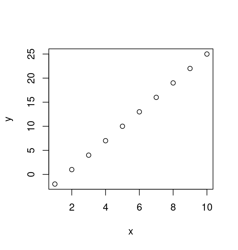
3.2.7 Getting help
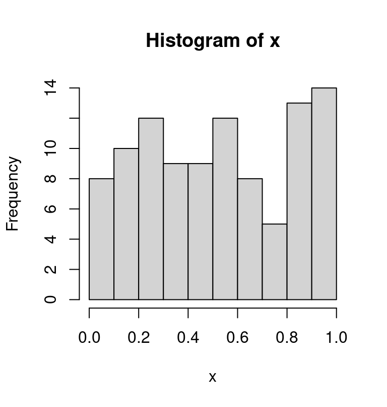
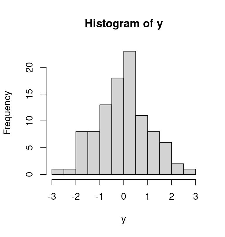
R has a lot of functions, and extra packages that can provides even more. It may seem a bit overwhelming, but it is very easy to get help about how to use a function: just type in a question mark, followed by the name of the function. For example, to see the help of the function we used above to generate the histogram, type
?hist\[\\[1in]\]