5 Linear models

This section will provide some worked examples of how to do analyses in R.

5.1 Simple linear regression

In this example² we will see how to import data into R and perform a simple linear regression analysis.

According to the standard big-bang model, the universe expands uniformly and locally, according to Hubble’s law³ \[ \text{velocity} = \beta \times \text{distance} \] where \(\text{velocity}\) and \(\text{distance}\) are the relative velocity and distance of a galaxy, respectively; and \(\beta\) is “Hubble’s constant”⁴. Note that this is a simple linear equation, in which \(\beta\) indicate how much the variable \(\text{velocity}\) changes for each unitary increase in the variable \(\text{distance}\).

According to this model \(\beta^{-1}\) gives the approximate age of the universe, but \(\beta\) is unknown and must somehow be estimated from observations of \(\text{velocity}\) and \(\text{distance}\), made for a variety of galaxies at different distances from us. Luckily we have available data from the Hubble Space Telescope. Velocities are assessed by measuring the Doppler effect red shift in the spectrum of light that we receive from the Galaxies. Distance is estimated more indirectly, by using the discovery that in certain class of stars (Cepheids), which display fluctuations in diameter and temperature over a stable period, there is a systematic relationship between the period and their luminosity.

We can load a dataset of measurements from the Hubble Space Telescope in R using the following code

d <- read.table(file="https://raw.githubusercontent.com/mattelisi/RHUL-stats/main/data/hubble.txt", 
                header=T)

read.table is a generic function to import dataset in text files (e.g. .csv files) into R. We use the argument header=T to specify that the first line of the dataset gives the names of the columns. Note that the argument file here is a URL, but it could be also a path to a file in our local folder. To see the help of this function, and what other arguments and features are available type ?read.table in the R command line.

We can use the command str() to examine what we have imported

str(d)
#> 'data.frame':    24 obs. of  3 variables:
#>  $ Galaxy  : chr  "NGC0300" "NGC0925" "NGC1326A" "NGC1365" ...
#>  $ velocity: int  133 664 1794 1594 1473 278 714 882 80 772 ...
#>  $ distance: num  2 9.16 16.14 17.95 21.88 ...

This tells us that our data frame has 3 variables:

Galaxy, the ‘names’ of the galaxies in the dataset
velocity, their relative velocity in Km/sec
distance, their distance expressed in Mega-parsecs⁵

We can plot⁶ them using the following code:

plot(d$distance, # indicate which variable on X axis
     d$velocity, # indicate which variable on Y axis
     xlab="Distance [Mega-parsecs]",
     ylab="Velocity [Km/sec]", 
     pch=19) # set the type of point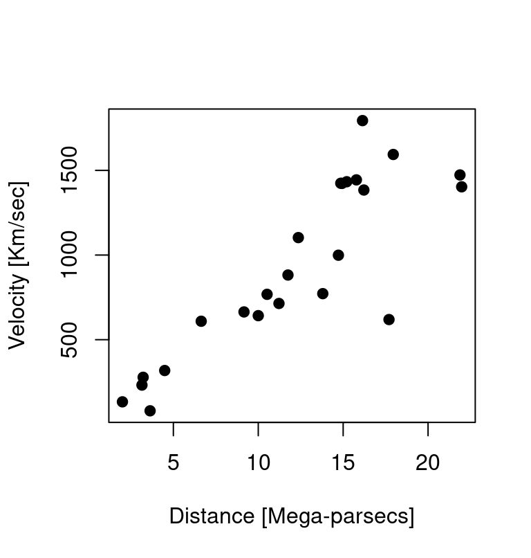

It is clear, from the figure, that the observed data do not follow Hubble’s law exactly, but given the how these measurements were obtained (there is uncertainty about the true values of the distance and velocities) it would be surprising if they did. Given the apparent variability, what can be inferred from these data? In particular:

what value of \(\beta\) is most consistent with the data?
what range of \(\beta\) values is consistent with the data?

In order to make inferences we make some assumptions about the nature of the measurement noise. Specifically, we assume that measurements errors are well-characterized by a Gaussian distribution. This result in the following model: \[\begin{align*} y &= \beta x + \epsilon \\ \epsilon &\sim \mathcal{N} \left(0, \sigma_{\epsilon}^2 \right) \end{align*}\] which is essentially a linear regression but without the intercept: that is, whereas normally a linear regression model include an additive term that is not multiplied with the predictor (as in \(y = \beta_0 + \beta_1 x + \epsilon\)), which gives the expected value of the dependent variable when all predictors are set to zero, in this case the theory tells us we can assume the intercept (the term \(\beta_0\)) is zero and we can ignore it.

We can fit the model with the function lm in R. Note that to tell R that I don’t want to fit the intercept, I include in the formula the term 0 + - this essentially tells R that the intercept term is set to zero⁷

hub.m <- lm(velocity ~ 0 + distance, d)
summary(hub.m)
#> 
#> Call:
#> lm(formula = velocity ~ 0 + distance, data = d)
#> 
#> Residuals:
#>    Min     1Q Median     3Q    Max 
#> -736.5 -132.5  -19.0  172.2  558.0 
#> 
#> Coefficients:
#>          Estimate Std. Error t value Pr(>|t|)    
#> distance   76.581      3.965   19.32 1.03e-15 ***
#> ---
#> Signif. codes:  
#> 0 '***' 0.001 '**' 0.01 '*' 0.05 '.' 0.1 ' ' 1
#> 
#> Residual standard error: 258.9 on 23 degrees of freedom
#> Multiple R-squared:  0.9419, Adjusted R-squared:  0.9394 
#> F-statistic: 373.1 on 1 and 23 DF,  p-value: 1.032e-15

So, based on this data, our estimate of the Hubble constant is 76.58 with a standard error of 3.96. The standard error - which is the standard deviation of the sampling distribution of our estimates - gives an ideas of the range of values that is compatible with our data and could be used to compute a confidence intervals (roughly, we would expect that the ‘true’ values of the parameters lies in the interval defined by \(\pm\) 2 standard errors 95% of the times).

So, how old is the universe?

The Hubble constant estimate have units of \(\frac{\text{Km}/\text{sec}}{\text{Mega-parsecs}}\). A Mega-parsecs is \(3.09 \times 10^{19} \text{Km}\), so we divide our estimate of \(\hat \beta\) by this amount. The reciprocal of \(\hat \beta\) then gives the approximate age of the universe (in seconds). In R we can calculate it (in years) as follow

# transform in Km
hubble.const <- coef(hub.m)/(3.09 * 10^(19))

# invert to get age in seconds
age <- 1/hubble.const

# use unname() to avoid carrying over 
# the label "distance" from the model
age <- unname(age)

# transform age in years
age <- age/(60^2 * 24 * 365)

# age in billion years
age/10^9
#> [1] 12.79469

giving an estimate of about 13 billion years.

4 Correlations

6 Models for count data