10 Multilevel Bayesian models
10.1 Overdispersed poisson GLMM example: police stops in NYC
In this section, we analyze an example dataset of police stop-and-frisk data, referred to in police_BDA3rd_p435.pdf available at this repository.
The data contains counts of stops by precinct, ethnicity, and crime type, along with population and DCJS arrests.
We’ll fit an overdispersed Poisson regression with random intercepts by precinct and an observation-level random effect, following Gelman & Hill’s approach.
10.1.1 1. Load and Explore the Data
# Read the data from a text file
d <- read_delim("../data/police_stops.txt", delim = " ", col_names = TRUE)

# Examine the structure
str(d)
#> spc_tbl_ [900 × 6] (S3: spec_tbl_df/tbl_df/tbl/data.frame)
#>  $ stops       : num [1:900] 75 36 74 17 37 39 23 3 26 32 ...
#>  $ pop         : num [1:900] 1720 1720 1720 1720 1368 ...
#>  $ past.arrests: num [1:900] 191 57 599 133 62 27 149 57 135 16 ...
#>  $ precinct    : num [1:900] 1 1 1 1 1 1 1 1 1 1 ...
#>  $ eth         : num [1:900] 1 1 1 1 2 2 2 2 3 3 ...
#>  $ crime       : num [1:900] 1 2 3 4 1 2 3 4 1 2 ...
#>  - attr(*, "spec")=
#>   .. cols(
#>   ..   stops = col_double(),
#>   ..   pop = col_double(),
#>   ..   past.arrests = col_double(),
#>   ..   precinct = col_double(),
#>   ..   eth = col_double(),
#>   ..   crime = col_double()
#>   .. )
#>  - attr(*, "problems")=<externalptr>
# Note:
# precincts are numbered 1-75
# ethnicity 1=black, 2=hispanic, 3=white
# crime type 1=violent, 2=weapons, 3=property, 4=drug
10.1.2 2. Summary Statistics
We’ll group by ethnicity to see how many stops, how many arrests, and what fraction of population each group represents across all precincts/crime categories.
d_summaries <- d %>%
  mutate(eth = case_when(
    eth == 1 ~ "black",
    eth == 2 ~ "hispanic",
    eth == 3 ~ "white"
  )) %>%
  group_by(eth) %>%
  summarise(
    pop           = sum(pop),
    total_stops   = sum(stops),
    total_arrests = sum(past.arrests),
    .groups = "drop"
  ) %>%
  mutate(
    prop_of_all_stops = total_stops / sum(total_stops),
    pop_fraction      = pop / sum(pop)
  )

d_summaries
#> # A tibble: 3 × 6
#>   eth        pop total_stops total_arrests prop_of_all_stops
#>   <chr>    <dbl>       <dbl>         <dbl>             <dbl>
#> 1 black   7.46e6       69823        125719             0.531
#> 2 hispan… 6.93e6       44623         74898             0.340
#> 3 white   1.27e7       16974         35922             0.129
#> # ℹ 1 more variable: pop_fraction <dbl>
10.1.3 3. Model Definition
We define the overdispersed Poisson model:
\[ y_{ep} \;\sim\; \text{Poisson}\bigl(\underbrace{\text{past.arrests}_{ep} \times \tfrac{15}{12}}_{\text{offset term}} \;\times\; e^{\,\alpha_{e} + \beta_{p} + \epsilon_{ep}} \bigr), \]
where:
-
\(y_{ep}\) = number of stops for ethnicity \(e\) in precinct \(p\).
-
\(\alpha_{e}\) = fixed effect for each ethnicity (\(e = 1,2,3\)).
-
\(\beta_{p}\) = random effect for precinct \(p\), with \(\beta_p \sim N(0, \sigma_\beta^2).\)
- \(\epsilon_{ep}\) = observation-level overdispersion, \(\epsilon_{ep} \sim N(0, \sigma_\epsilon^2).\)
Hence, the log-rate is: \(\log(\lambda_{ep}) = \alpha_e + \beta_p + \epsilon_{ep}\), and we multiply \(\lambda_{ep}\) by the offset \(\text{past.arrests}_{ep} \times \tfrac{15}{12}\).
10.1.3.1 Non-Centered Parametrization
We call \(\beta_p\) non-centered if we write:
\[ \beta_p = \sigma_\beta \;\beta_{\text{raw},p}, \quad \beta_{\text{raw},p} \sim N(0,1), \]
instead of sampling \(\beta_p\) directly from \(N(0,\sigma_\beta^2)\). This often improves sampling efficiency in hierarchical models. The same logic applies to \(\epsilon_{ep}\).
10.1.4 4. Stan Code
Below is the Stan code (which you can save in a file named overdispersed_poisson.stan):
data {
  int<lower=1> N;          // total # of (eth, precinct) data points
  int<lower=1> n_eth;      // number of ethnicity categories, e.g. 3
  int<lower=1> n_prec;     // number of precincts

  int<lower=0> y[N];       // outcome counts y_{ep}
  vector[N] past_arrests;  // baseline/reference rate

  int<lower=1, upper=n_eth> eth[N];      // ethnicity ID for each row
  int<lower=1, upper=n_prec> precinct[N]; // precinct ID for each row
}

parameters {
  // Ethnicity effects (fixed)
  vector[n_eth] alpha;

  // Random intercepts for precinct
  real<lower=0> sigma_beta;
  vector[n_prec] beta_raw;   // non-centered param for precinct

  // Overdispersion
  real<lower=0> sigma_eps;
  vector[N] eps_raw;         // non-centered param for each (e,p) observation
}

transformed parameters {
  vector[n_prec] beta;
  beta = sigma_beta * beta_raw;

  vector[N] eps;
  eps = sigma_eps * eps_raw;
}

model {
  // Priors (adjust as appropriate)
  alpha ~ normal(0, 5);
  sigma_beta ~ exponential(1);
  beta_raw ~ normal(0, 1);

  sigma_eps ~ exponential(1);
  eps_raw ~ normal(0, 1);

  // Likelihood
  for (i in 1:N) {
    // lambda = alpha[ eth[i] ] + beta[ precinct[i] ] + eps[i]
    // Multiply by (past_arrests[i] * 15/12) to get Poisson mean
    y[i] ~ poisson(past_arrests[i] * (15.0 / 12.0) * exp(alpha[eth[i]] + beta[precinct[i]] + eps[i]));
  }
}
10.1.5 5. Prior Predictive Check
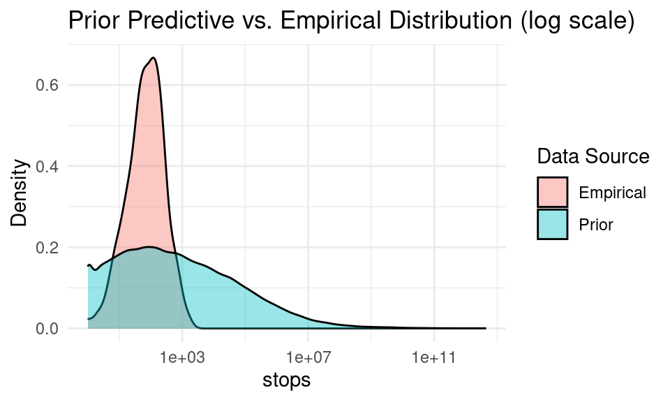
Before fitting the model, it’s good practice to simulate data under the prior to see if the implied distribution is reasonable. For brevity, here’s a minimal example:
# Suppose we do a quick simulation from the prior in R:
# (We won't run Stan's generated quantities block, but just do a rough check.)

set.seed(123)
N_sim <- 10
sigma_beta_sim <- rexp(1, 1)
sigma_eps_sim <- rexp(1, 1)
alpha_sim <- rnorm(3, 0, 5) # 3 ethnicity groups

beta_raw_sim <- rnorm(75, 0, 1)
beta_sim <- sigma_beta_sim * beta_raw_sim

eps_raw_sim <- rnorm(N_sim, 0, 1)
eps_sim <- sigma_eps_sim * eps_raw_sim

cat("Simulated sigma_beta =", sigma_beta_sim, "\n")
#> Simulated sigma_beta = 0.8434573
cat("Simulated sigma_eps  =", sigma_eps_sim, "\n")
#> Simulated sigma_eps  = 0.5766103
cat("Simulated alpha =", alpha_sim, "\n")
#> Simulated alpha = -1.150887 7.793542 0.352542
We could draw some random past_arrests values (e.g., 1–50) and see how big the Poisson means might get. If these are unreasonably large or small, we might tighten the priors.
10.1.6 6. Fit the Model
Important: If past.arrests == 0 for some rows but stops are nonzero, we need to avoid a zero Poisson mean. One quick fix is to add a small constant (e.g. 0.5) to past.arrests.
# Correction for zero arrests
d$past.arrests <- ifelse(d$past.arrests == 0, 0.5, d$past.arrests)10.1.6.2 Compile and Run Stan
# Make sure you have the Stan model saved as "overdispersed_poisson.stan".
# Then run:
fit <- stan(
  file = "../models/overdispersed_poisson.stan",
  data = stan_data,
  iter = 2000,
  chains = 4,
  cores = 4
)
print(fit, pars = c("alpha", "sigma_beta", "sigma_eps"))
#> Inference for Stan model: anon_model.
#> 4 chains, each with iter=2000; warmup=1000; thin=1;
#> post-warmup draws per chain=1000, total post-warmup draws=4000.
#>
#>             mean se_mean   sd  2.5%   25%   50%   75% 97.5%
#> alpha[1]   -0.58       0 0.09 -0.76 -0.64 -0.58 -0.52 -0.41
#> alpha[2]   -0.53       0 0.09 -0.71 -0.59 -0.53 -0.47 -0.34
#> alpha[3]   -0.97       0 0.09 -1.15 -1.03 -0.97 -0.91 -0.80
#> sigma_beta  0.54       0 0.06  0.43  0.50  0.54  0.58  0.68
#> sigma_eps   1.11       0 0.03  1.06  1.10  1.11  1.13  1.17
#>            n_eff Rhat
#> alpha[1]    7809    1
#> alpha[2]    6275    1
#> alpha[3]    7447    1
#> sigma_beta  1065    1
#> sigma_eps   1688    1
#>
#> Samples were drawn using NUTS(diag_e) at Tue Mar 25 16:31:01 2025.
#> For each parameter, n_eff is a crude measure of effective sample size,
#> and Rhat is the potential scale reduction factor on split chains (at
#> convergence, Rhat=1).
Here, alpha are the ethnic-group log-effects, sigma_beta is the precinct-level standard deviation, and sigma_eps is the overdispersion. You can also examine random intercepts beta or the eps in detail.
10.1.7 7. Diagnostic Checks
# Traceplots
traceplot(fit, pars = c("alpha", "sigma_beta", "sigma_eps"))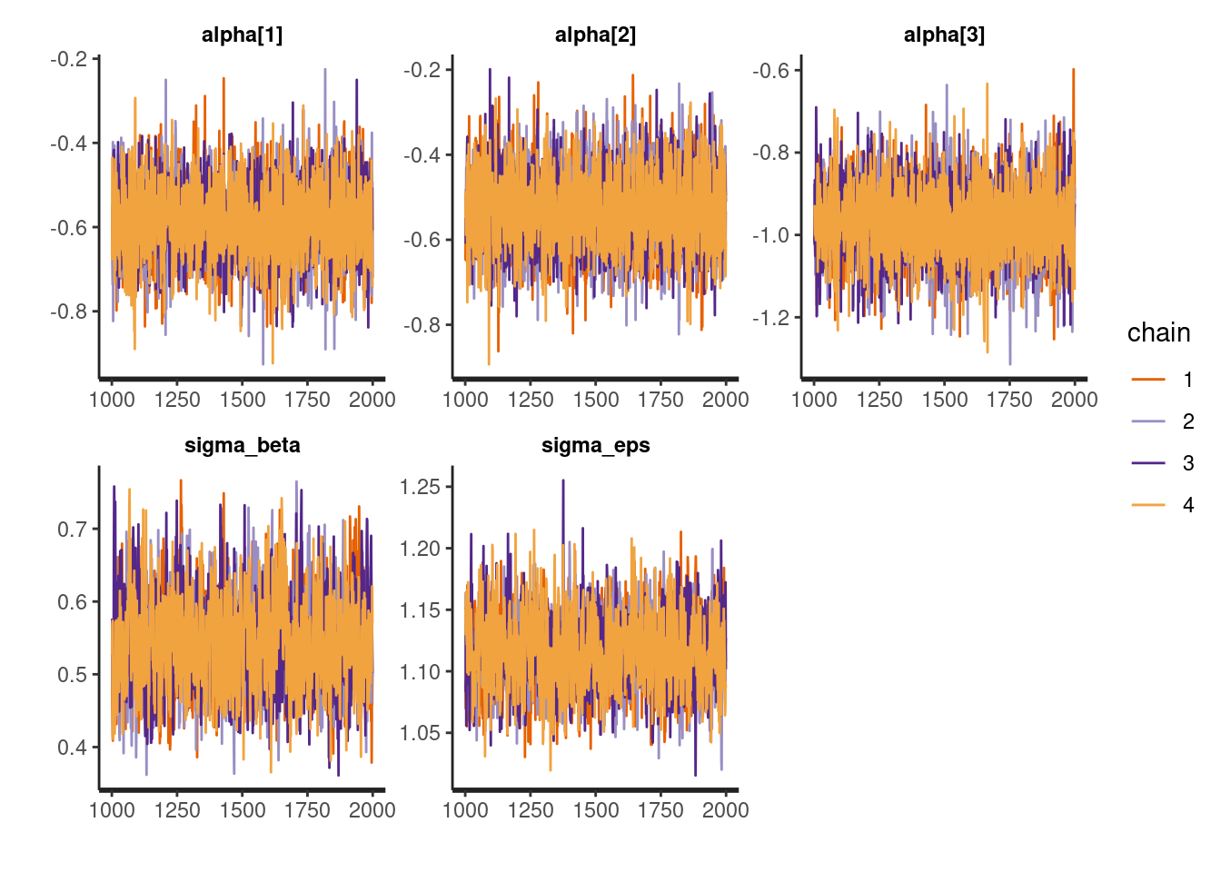
# Pairs plot for some key parameters
pairs(fit, pars = c("alpha[1]", "alpha[2]", "alpha[3]", "sigma_beta", "sigma_eps"))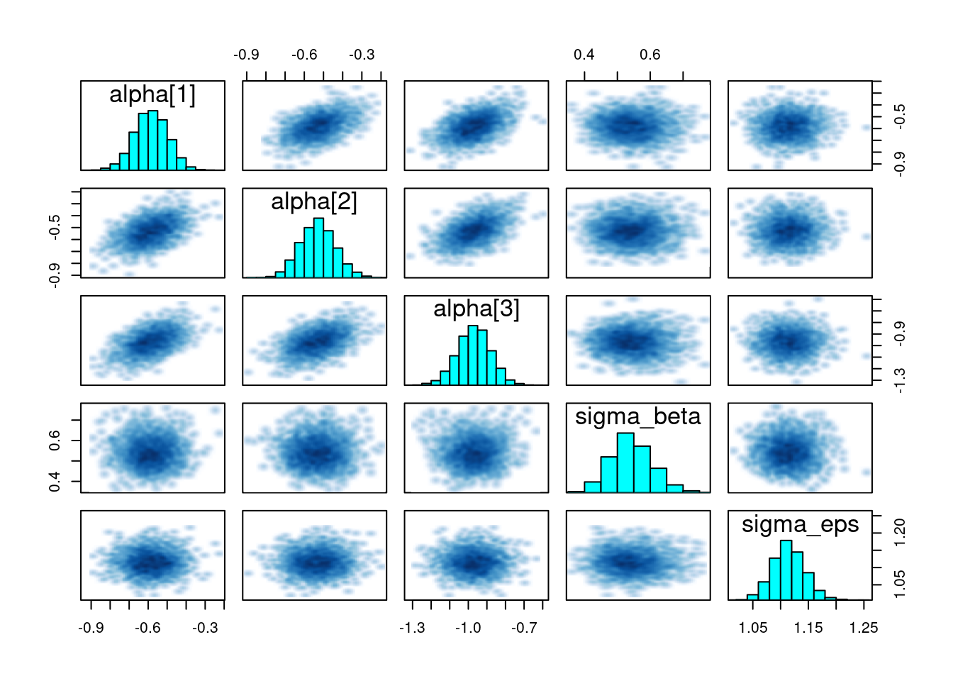
Check for good mixing (no major issues in traceplots) and no suspicious funnel shapes in pairs plots.
10.1.8 8. Posterior Analysis
We use tidybayes to extract samples and summarize. Suppose we want to look at the exponentiated ethnic effects (relative stops vs. arrests).
library(tidybayes)

posterior <- fit %>%
  spread_draws(alpha[e]) %>%
  mutate(rate = exp(alpha))  # exponentiate to interpret as a multiplicative factor

# Summarize the rate by ethnicity
posterior %>%
  group_by(e) %>%
  mean_hdi(rate, .width = 0.95)
#> # A tibble: 3 × 7
#>       e  rate .lower .upper .width .point .interval
#>   <int> <dbl>  <dbl>  <dbl>  <dbl> <chr>  <chr>
#> 1     1 0.560  0.467  0.660   0.95 mean   hdi
#> 2     2 0.591  0.488  0.697   0.95 mean   hdi
#> 3     3 0.381  0.316  0.449   0.95 mean   hdi
If e=1 = black, e=2 = hispanic, e=3 = white, these give the average ratio of stops to arrests (relative to some baseline) for each ethnicity, controlling for precinct and overdispersion.
You might then compare black vs. white, etc., by calculating differences or ratios in the posterior draws.
posterior_ratios <- posterior %>%
pivot_wider(
id_cols = c(.chain, .iteration, .draw), # these 3 columns identify each draw
names_from = e, # which column to pivot on
values_from = rate, # which column holds the values
names_prefix = "eth_"
) %>%
mutate(
black_vs_white = eth_1 / eth_3,
hisp_vs_white = eth_2 / eth_3
) %>%
# Pivot longer so each ratio is in its own row
pivot_longer(
cols = c(black_vs_white, hisp_vs_white),
names_to = "contrast",
values_to = "ratio"
) %>%
# Summarize with mean_hdi -> returns columns .mean, .lower, .upper
group_by(contrast) %>%
mean_hdi(ratio, .width = 0.95)
posterior_ratios
#> # A tibble: 2 × 7
#> contrast ratio .lower .upper .width .point .interval
#> <chr> <dbl> <dbl> <dbl> <dbl> <chr> <chr>
#> 1 black_vs_white 1.48 1.22 1.75 0.95 mean hdi
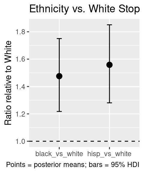
#> 2 hisp_vs_white 1.56 1.28 1.85 0.95 mean hdiThis gives an estimate of how many times more likely black (or hispanic) stops are relative to white stops, after controlling for arrests, precinct differences, and overdispersion.
We can use this for plotting e.g.:
ggplot(posterior_ratios, aes(x = contrast, y = ratio)) +
  geom_point(size=3) +
  geom_hline(yintercept=1, lty=2)+
  geom_errorbar(aes(ymin = .lower, ymax = .upper), width = 0.1) +
  labs(
    x = NULL,
    y = "Ratio relative to White",
    title = "Ethnicity vs. White Stop Ratios",
    caption = "Points = posterior means; bars = 95% HDI"
  )
10.1.9 Prior predictive check
N <- nrow(d)
n_eth <- length(unique(d$eth))
n_prec <- length(unique(d$precinct))

# Decide how many draws from the prior to simulate
n_sims <- 200

# We'll store all simulated Y values in a single big vector
# so we can compare them to the observed distribution
all_prior_stops <- numeric(0)

set.seed(101)  # reproducibility

for (s in 1:n_sims) {

  # 1) Sample the parameters from their priors


  alpha_draw <- rnorm(n_eth, mean = 0, sd = 5) # alpha: one for each ethnicity
  sigma_beta_draw <- rexp(1, rate = 1)
  beta_raw_draw <- rnorm(n_prec, 0, 1)
  beta_draw <- sigma_beta_draw * beta_raw_draw

  sigma_eps_draw <- rexp(1, rate = 1)          # Overdispersion
  eps_raw_draw <- rnorm(N, 0, 1)
  eps_draw <- sigma_eps_draw * eps_raw_draw

  # 2) Generate y (stops) from Poisson for each observation i

  past_arrests_offset <- ifelse(d$past.arrests == 0, 0.5, d$past.arrests)

  # compute the linear predictor for each row i
  lambda_vec <- numeric(N)
  for (i in seq_len(N)) {
    e <- d$eth[i]
    p <- d$precinct[i]
    lambda_vec[i] <- alpha_draw[e] + beta_draw[p] + eps_draw[i]
  }

  # Poisson means
  mu_vec <- past_arrests_offset * (15/12) * exp(lambda_vec)

  # sample from Poisson
  y_sim <- rpois(N, mu_vec)

  # 3) Store in a big vector for later comparison
  all_prior_stops <- c(all_prior_stops, y_sim)
}

# Now we have n_sims * N simulated 'stops' from the prior
# Compare with the empirical distribution:
observed_stops <- d$stops

df_plot <- tibble(
  value = c((observed_stops ), (all_prior_stops )),
  type  = rep(c("Empirical", "Prior"), c(length(observed_stops), length(all_prior_stops)))
)

# Plot densities
ggplot(df_plot, aes(x = value, fill = type)) +
  geom_density(alpha = 0.4) +
  labs(
    x = "stops",
    y = "Density",
    title = "Prior Predictive vs. Empirical Distribution (log scale)",
    fill = "Data Source"
  ) +
  theme_minimal()+
  scale_x_log10()