7 Models for ordinal data

Ordinal-type of variable arise often in psychology. One common example are responses to Likert scales. Although it is very common practice that these are analyzed with a linear model, it is know that this approach can lead to serious inference errors.¹⁷ For this reason, the recommended approach is to use a model appropriate for ordinal data. Here I will describe an approach to this, using an ordered logistic regression model (also know as proportional odds model).

7.1 Ordered logistic regression

One way to think about this model is by assuming the existence of a continuous latent quantity, call it \(y\), specified by a logistic probability density function. The latent distribution is partitioned into a series of \(k\) intervals, where \(k\) is the number of ordered choice options available to respondents, using \(k+1\) latent cut-points, \(c_1, \ldots, c_{k+1}\). By integrating the latent density function within each interval we obtain the ordinal response probabilities \(p_1, \ldots, p_k\). Other choices are possible (e.g. assuming a normally distributed latent variable would yield an ordered probit model). Beyond mathematical convenience, one advantage of the ordered logit is that coefficient can be interpreted as ordered log-odds, implementing the proportional odds assumption.¹⁸

Formally, the model can be notated as

\[ \begin{aligned} p_k & = p\left(c_{k-1} < y \le c_k \mid \mu \right)\\ & = \text{logit}^{-1}\left(c_k - \mu \right) - \text{logit}^{-1}\left(c_{k-1} - \mu \right) \end{aligned} \]

where \[ \text{logit}^{-1}(\alpha) = \frac{1}{1+e^{-\alpha}} \] is the cumulative function of the logistic distribution (also known as inverse-logit), and \[ \mu = \beta_1 x_1 + \ldots + \beta_n x_n \] is the linear part of the model (a linear combination of the \(n\) predictor variables).

This is the general approach and the formalism used - below I present few examples that illustrates how this work in practice in R.

7.1.1 Mixed-effects ordinal regression

R libraries used in this example

library(ggplot2)
library(ordinal)
library(tidyverse)
library(DescTools)

In addition to the above libraries, here I will create a handy R function that gives the probabilities of the categorical responses given a mean value of the latent quantity (indicated with \(\mu\) above) and a set of cutpoints \(c_1, \ldots, c_{k+1}\). This will be used both for simulating the data and for plotting the fit of the model.

ordered_logistic <- function(eta, cutpoints){
  cutpoints <- c(cutpoints, Inf)
  k <- length(cutpoints)
  p <- rep(NA, k)
  p[1] <- plogis(cutpoints[1], location=eta, scale=1, lower.tail=TRUE)
  for(i in 2:k){
    p[i] <- plogis(cutpoints[i], location=eta, scale=1, lower.tail=TRUE) - 
      plogis(cutpoints[i-1], location=eta, scale=1, lower.tail=TRUE)
  }
  return(p)
}

For this example we simulate some data. We have two predictors: x1, a continuous predictor that vary with each observation, and d1 a dummy variable that indicate a categorical predictor with 2 levels (e.g. two experimental conditions). The conditions are within-subject, meaningthat each participant (identified by the variable id) is being tested in both conditions.

set.seed(5)
N <- 200
N_id <- 10
dat <- data.frame(
  id = factor(sample(1:N_id,N, replace = T)),
  d1 = rbinom(N,1,0.5), # dummy variable (0,1) indicate 2 conditions
  x1 = runif(n = N, min = 1, max = 10)
)
rfx <- rnorm(length(unique(dat$id)), mean=0, sd=5)
LP <- 0.5*dat$x1 + 2*dat$d1 + rfx[dat$id]
for(i in 1:N){
  dat$response[i] <- which(rmultinom(1,1, ordered_logistic(LP[i], c(0,2.5, 5,10)))==1)
}
dat$response <- factor(dat$response)
str(dat)
#> 'data.frame':    200 obs. of  4 variables:
#>  $ id      : Factor w/ 10 levels "1","2","3","4",..: 2 9 9 9 5 7 7 3 3 6 ...
#>  $ d1      : int  0 0 0 0 0 0 0 1 0 0 ...
#>  $ x1      : num  6.81 1.49 6.94 3.09 3.97 ...
#>  $ response: Factor w/ 5 levels "1","2","3","4",..: 4 1 3 2 2 3 3 4 3 2 ...

The dependent variable is categorical with 5 levels - here is a plot of the number of responses per category in the two conditions. We are interested in testing whether the distribution differ across the conditions.

ggplot(dat,aes(x=response))+
  geom_bar()+
  facet_grid(.~d1)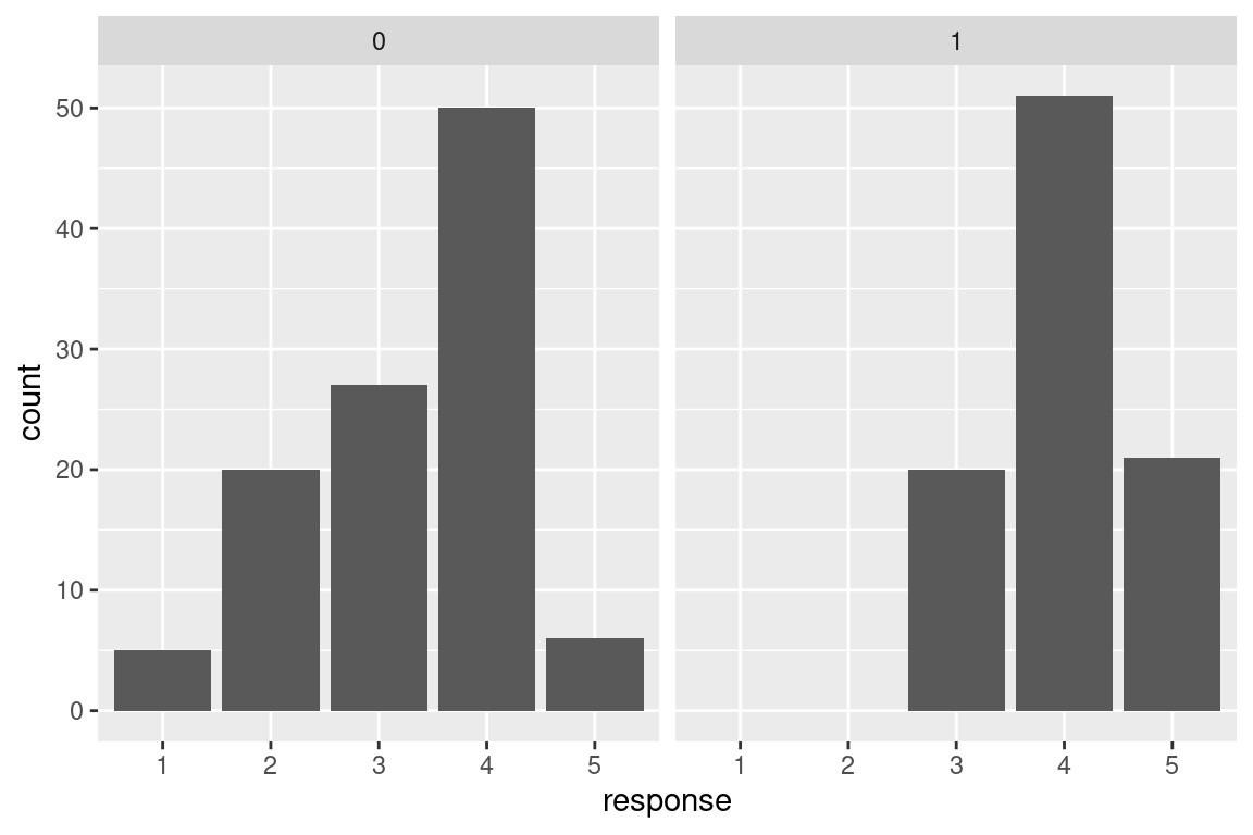

We use the clmm() function in the package ordinal to estimate the model. The syntax is similar to what we would use for a linear mixed effect model. Note that in the output the Threshold coefficients are the latent cutpoints \(c_1, \ldots, c_{4}\)

model <- clmm(response ~ x1 + d1 + (1|id), data = dat)
summary(model)
#> Cumulative Link Mixed Model fitted with the Laplace approximation
#> 
#> formula: response ~ x1 + d1 + (1 | id)
#> data:    dat
#> 
#>  link  threshold nobs logLik  AIC    niter    max.grad
#>  logit flexible  200  -175.75 365.49 291(919) 6.56e-05
#>  cond.H 
#>  8.6e+02
#> 
#> Random effects:
#>  Groups Name        Variance Std.Dev.
#>  id     (Intercept) 4.224    2.055   
#> Number of groups:  id 10 
#> 
#> Coefficients:
#>    Estimate Std. Error z value Pr(>|z|)    
#> x1  0.55685    0.07516   7.409 1.27e-13 ***
#> d1  2.29521    0.36659   6.261 3.82e-10 ***
#> ---
#> Signif. codes:  
#> 0 '***' 0.001 '**' 0.01 '*' 0.05 '.' 0.1 ' ' 1
#> 
#> Threshold coefficients:
#>     Estimate Std. Error z value
#> 1|2  -2.1850     0.8512  -2.567
#> 2|3   0.2853     0.7664   0.372
#> 3|4   2.9453     0.8059   3.655
#> 4|5   7.8126     1.0072   7.757

There is no function that can out-of the box calculate the predictions of the model for us, so this will need some coding. I also use the library DescTools to calculate simultaneous multinomial confidence intervals. In the resulting plot the black line are model fit, and bar the observed responses.

# pre-allocate a matrix to store model predictions
# note that these are a vector of 5 probabilities for each trial
pred_mat <- matrix(NA, nrow=N, ncol=length(unique( dat$response)))

for(i in 1:N){
  
  # first calculate the linear predictor 
  # by summing all variable as indicated
  # in the model formulate, weighted by the coefficients
  eta <- dat$x1[i]*model$beta['x1'] +  dat$d1[i]*model$beta['d1'] + model$ranef[dat$id[i]]
  # note that + model$ranef[dat$id[i]] adds 
  # the random intercept for the subjects of observation i
  
  # calculate vector of predicted probabilities
  pred_mat[i,] <- ordered_logistic(eta, model$Theta)
  
}

# add predictions to dataset
pred_dat <- data.frame(pred_mat)
colnames(pred_dat) <- paste("resp_",1:ncol(pred_mat),sep="")
pred_dat <- cbind(dat, pred_dat)

# in order to visalize the predictions, 
# we first average them for each condition
pred_dat %>%
  pivot_longer(cols=starts_with("resp_"), 
               names_prefix="resp_",
               values_to = "prob",
               names_to ="response_category") %>%
  group_by(d1, response_category) %>%
  summarise(prob = mean(prob),
            n=sum(response==response_category)) %>%
  group_by(d1) %>%
  mutate(prop_obs = n/sum(n),
    response=as.numeric(response_category)) -> pred_d1
#> `summarise()` has grouped output by 'd1'. You can override
#> using the `.groups` argument.

# cimpute the multinomial interval
pred_d1$CI_lb <- MultinomCI(pred_d1$n)[,"lwr.ci"] *2 
pred_d1$CI_ub <- MultinomCI(pred_d1$n)[,"upr.ci"] *2
# note that I multiply for 2 because in the plot each condition 
# will be in a different panel and the probability will sum to 1 in each panel

# visualize (aggregated) ordinal response & prediction
# the black line are the predictions of the model

ggplot(pred_d1,aes(x=response, y=prop_obs))+
  geom_col()+
  geom_errorbar(data=pred_d1, aes(ymin=CI_lb, ymax=CI_ub),width=0.2)+
  facet_grid(.~d1)+
  geom_line(data=pred_d1, aes(y=prob), size=2)+
  labs(y="probability")
#> Warning: Using `size` aesthetic for lines was deprecated in ggplot2
#> 3.4.0.
#> ℹ Please use `linewidth` instead.
#> This warning is displayed once every 8 hours.
#> Call `lifecycle::last_lifecycle_warnings()` to see where
#> this warning was generated.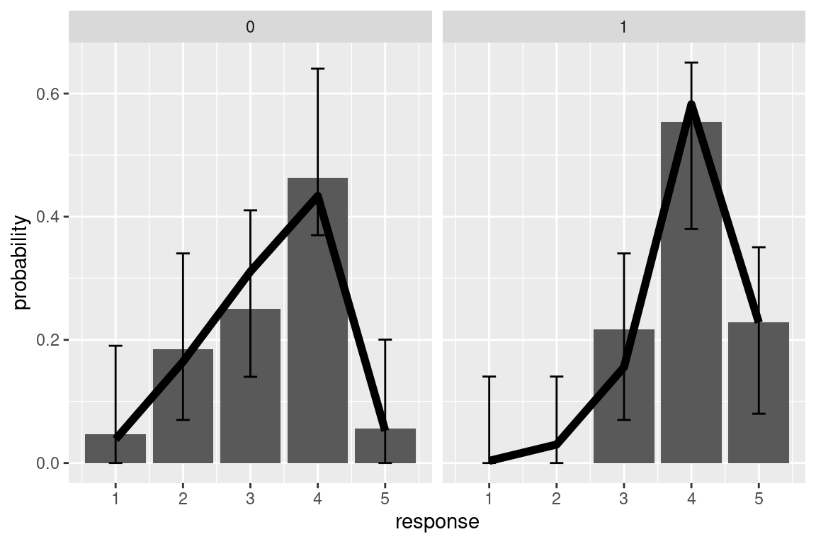

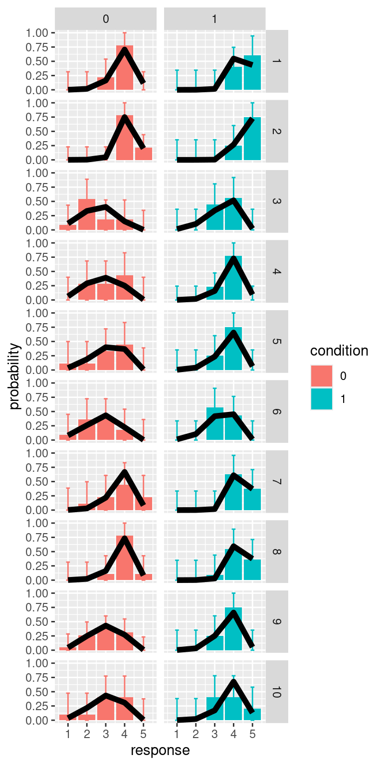
We can repeat the same process also for calculating predictions for individual participants

# split by ID
pred_dat %>%
  pivot_longer(cols=starts_with("resp_"), 
               names_prefix="resp_",
               values_to = "prob",
               names_to ="response_category") %>%
  group_by(id, d1, response_category) %>%
  summarise(prob = mean(prob),
            n=sum(response==response_category)) %>%
  group_by(d1, id) %>%
  mutate(prop_obs = n/sum(n),
         response=as.numeric(response_category))  -> pred_d1
#> `summarise()` has grouped output by 'id', 'd1'. You can
#> override using the `.groups` argument.

# calculate multinomial CI
# we do a loop over all participants and conditions
pred_d1$CI_lb <- NA
pred_d1$CI_ub <- NA
for(i in unique(pred_d1$id)){
  for(cond in c(0,1)){
    pred_d1$CI_lb[pred_d1$id==i & pred_d1$d1==cond] <- DescTools::MultinomCI(pred_d1$n[pred_d1$id==i & pred_d1$d1==cond])[,"lwr.ci"] 
    pred_d1$CI_ub[pred_d1$id==i & pred_d1$d1==cond] <- DescTools::MultinomCI(pred_d1$n[pred_d1$id==i & pred_d1$d1==cond])[,"upr.ci"]
  }
}

pred_d1 %>%
  mutate(condition = factor(d1)) %>%
  ggplot(aes(x=response, y=prop_obs, fill=condition))+
    geom_col()+
    geom_errorbar(aes(ymin=CI_lb, ymax=CI_ub, color=condition), width=0.2)+
    facet_grid(id~d1)+
    geom_line(aes(y=prob), size=2)+
    labs(y="probability")

6 Models for count data

8 Meta-analyses